Table of Contents
Conventional model-based control in power electronics relies heavily on deriving precise mathematical models of the physical system. In contrast, data-driven control shifts this paradigm by estimating control laws directly from empirical data. A key example of this approach is Artificial Neural Network (ANN)-based control. ANNs serve as universal function approximators that extract complex input–output relationships directly from empirical or simulated datasets. Beyond mapping known parameters, ANNs are good at generalization, allowing them to accurately predict system behaviour across unseen operating conditions. This robustness is particularly advantageous for managing systems where the underlying dynamics are complex or defy explicit mathematical modelling. Additionally, their inherent structural flexibility makes them naturally suited for multi-variable systems [1]. While the foundational mathematics of ANNs were established in 1943, their application in power electronics has surged recently, becoming a dominant area of research [2].
This technical note aims to replace the traditional inner-loop discrete PI current regulator with a lightweight feedforward neural network (FNN), a form of supervised machine learning. The FNN is designed to accurately reproduce the voltage-reference mapping within a standard grid-following current control structure. Finally, this approach is validated by implementing the ANN-based controller on a physical TPI8032 programmable inverter.
Classification of ANNs
Depending on the learning task, ANNs are generally categorized into two main groups: classification and regression. Classification is used for discrete decisions, while regression handles continuous predictions. In power electronics, this distinction aligns perfectly with how the ANN drives the converter:
- Direct control (Classification): The ANN directly generates the discrete gate signals (e.g., ON/OFF) for the semiconductor switches. As the outputs are discrete states, this is formulated as a classification problem.
- Indirect control (Regression): The ANN calculates a continuous control variable, such as the voltage reference or duty cycle, which is then fed into a modulator. As the output is a continuous numerical value, this requires a regression model.
In this technical note, the ANN replaces a standard discrete PI current controller, meaning it needs to map a continuous voltage reference. Therefore, an indirect control strategy based on a regression ANN is implemented.
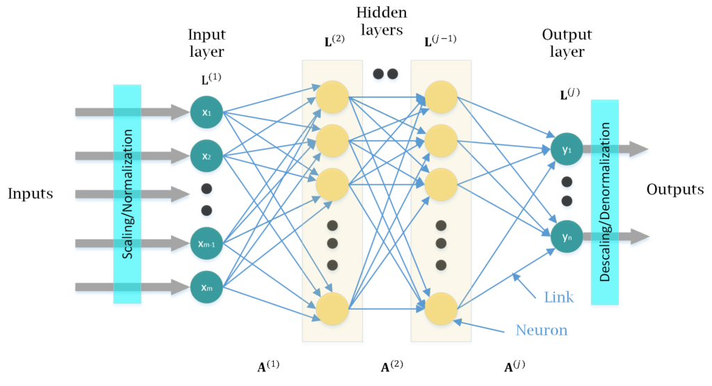
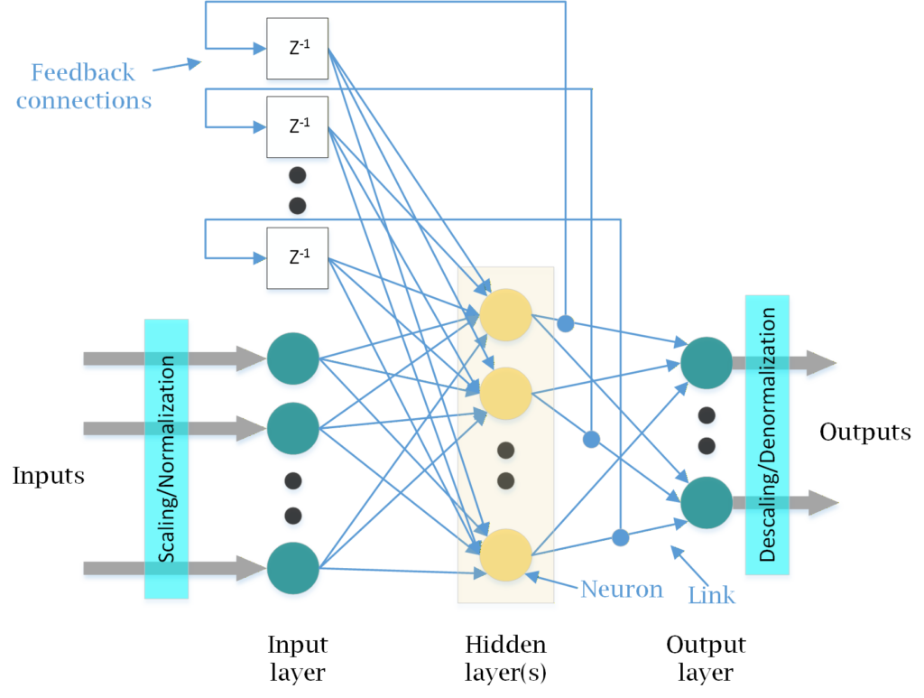
Beyond their learning task, ANNs can also be classified by their internal topology into feedforward and recurrent architectures. Feedforward neural networks (FNNs) process data strictly in one direction (see Fig. 1). As static, memoryless systems, FNNs lack an internal state and require past samples to be explicitly included in the input vector to account for historical data. Standard feedforward models include Multilayer Perceptrons, Radial Basis Function networks, and Convolutional Neural Networks. In contrast, recurrent networks, including LSTMs and GRUs, incorporate feedback loops that retain an internal memory of past inputs (see Fig. 2). This makes them highly effective for modeling dynamic, time-dependent systems [3].
From all of these available ANN architectures, the Multilayer Perceptron (MLP) FNN is frequently adopted as a baseline due to its simplicity and implementation efficiency and is widely used in industrial applications [1]. Therefore, for this technical note, the MLP-FNN is selected for its strictly feedforward architecture, which ensures deterministic, low-latency execution required for a high-bandwidth controller. Additionally, its capability as a universal function approximator allows it to accurately reproduce the PI controller’s input-output mapping with minimal computational overhead.
MLP-FNN architecture
An MLP-FNN architecture typically comprises an input layer, one or more hidden layers, and an output layer, each containing one or multiple interconnected neurons, as illustrated in Fig. 1. Within each neuron, incoming signals are multiplied by their respective connection weights (\(w\)), which represent the strength of the input, summed together, and then shifted by a bias term (\(b\)). Finally, the aggregated value is passed through an activation function to generate the neuron’s output signal. This function is a mathematical operation that can include non-linearity, allowing the network to learn and model complex patterns beyond simple linear relationships. By iteratively adjusting the weights and biases during the training phase, the FNN encodes the learned relationships, enabling it to generalize accurately across its intended operating region [3].
Important concepts related to ANNs in general, and FNNs in particular, are detailed below:
Mathematical representation of FNN
Referring to Fig. 1, let the input vector be , and the output vector be
A typical mathematical expression for the output of neuron in layer :
where is the weight connecting neuron in layer to neuron in layer , is an offset, is the number of neurons in the preceding layer, and ( ⋅ ) is the activation function of layer .
Activation functions
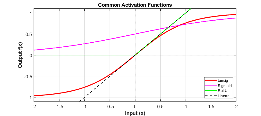
To enable the network to learn complex non-linear mappings, the neurons must utilize non-linear activation functions. For the network to be compatible with standard network training algorithms, these activation functions must be differentiable or piecewise differentiable. Among the various options available, the Rectified Linear Unit (ReLU) is the most commonly used due to its computational efficiency and effectiveness in mitigating gradient-related issues during training [4]. Fig. 3 illustrates some important activation functions commonly used in ANNs.
Network topology and design flexibility
FNN offers a significant degree of design flexibility. While the dimensionality of the input and output layers is typically determined by the physical system, the internal structure is largely user-defined. Key design choices include the number of hidden layers (depth), the number of neurons per layer (width), and the connectivity scheme (e.g., all-to-all vs. sparsified connections). Specifically, increasing the network’s depth enables it to learn highly complex, hierarchical abstractions of the data, while expanding its width allows it to capture a broader array of features at each processing stage. However, a model with excessive depth or width risks overfitting and needlessly inflating the execution time. Ultimately, this architectural freedom allows the user to carefully balance model learning capacity against the strict computational constraints of the physical application [4].
Training algorithms
The training algorithm used to calculate the network’s weight matrix depends on the architecture’s complexity. For simple, single-layer networks with linear input-output relationships, analytical methods such as the Pseudo-inverse or LASSO can be used for the direct optimization of the weights and biases. However, for multi-layer ANNs utilizing non-linear activation functions, iterative optimization methods are required.
Central to this iterative process is the loss function, which quantifies the error between the model’s predictions and the actual target values. Its primary function is to guide the optimization process, which iteratively adjusts the network’s weights and bias to minimize the error and improve the model’s accuracy.
The process of minimizing the loss in MLP-FNNs relies on two complementary phases: calculating the error gradients and updating the network weights and biases:
- Backpropagation is a computational algorithm that calculates the gradients of the loss function with respect to each weight by propagating the error information backward through the layers using the chain rule.
- Optimization algorithms use those calculated gradients to update the network parameters. While Stochastic Gradient Descent is a common first-order optimizer that takes steps in the direction of the steepest descent, second-order methods like the Levenberg-Marquardt algorithm are also widely used. Levenberg-Marquardt dynamically blends gradient descent with Gauss-Newton optimization, allowing for much faster convergence on moderate-sized problems.
Together, these mechanisms enable the network to learn from data. However, the speed and stability of this convergence are heavily influenced by the chosen hyperparameters. These hyperparameters are external configuration variables set before the training process begins, as opposed to parameters (weights and biases), which are learned during training. They govern the network’s structure (e.g., number of layers, number of neurons) and the learning process (e.g., learning rate, batch size) to optimize performance.
Data partitioning and validation
To ensure the model generalizes effectively to unseen operating conditions, the dataset is typically partitioned into three distinct subsets: training, validation, and testing. The training data is used directly by the algorithm to update the network’s weights and biases. While hyperparameters must be fixed before a training run begins, the validation data is used to evaluate the model’s performance under those specific settings, allowing the designer to iteratively tune the configuration across multiple independent runs. Finally, the test set provides a completely independent, unbiased evaluation of the final model to confirm its true performance on strictly unseen data.
During optimization, the training algorithm iterates through the data over several epochs, continuously adjusting the weights and biases to minimize the prediction error. This training process typically continues until the error on the validation set reaches a threshold and begins to increase. Halting the process at this exact point, a technique known as early stopping, is crucial to prevent the network from overfitting, thereby ensuring robust performance when deployed [4].
Challenges of ANN-based control
Implementing ANN-based control in converter applications presents several specific challenges:
- Data dependencies: The controller’s performance is intrinsically tied to the quality and breadth of the training dataset. Obtaining large, well-balanced datasets that cover the entire operating region, including rare events like faults, is often costly and time-consuming. Underrepresentation of these edge cases can lead to poor generalization.
- Design trade-offs and overfitting: Selecting the network architecture requires balancing accuracy against robustness. While increasing network depth and width enhances representational capacity, it raises computational costs and increases the risk of overfitting (learning noise rather than system dynamics). Cross-validation is essential to mitigate this risk [4].
- Verification and interpretability: Unlike standard linear controllers, ANNs often function as “black boxes” lacking analytical stability proofs. Consequently, safety-critical deployment typically requires auxiliary safety mechanisms, such as output saturations, runtime monitors, and fallback logic.
Experimental implementation of an ANN-based control
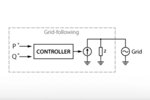
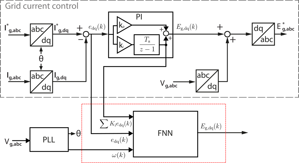
As an application example, an indirect MLP-FNN is implemented to regulate the output current of a three-phase grid-following converter. This example replaces the inner-loop PI current regulator with an offline-trained MLP-FNN. The deployment of the indirect FNN is performed at the controller interface, as shown in Fig. 4. The PLL synchronization, modulation (SVM), and protections remain unchanged, while the FNN reproduces the PI controller’s voltage-reference generation behavior.
Structure of FNN
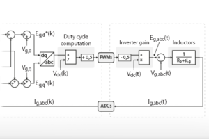
Instead of learning the full converter dynamics, the FNN is trained to emulate the mapping performed by the discrete PI current controller. At each control step , the FNN receives a set of controller-relevant input signals, and it outputs the corresponding voltage reference in dq coordinates. The input vector is constructed such that it captures the useful information that could be helpful for FNN in mapping the input vector to the output vector.
- Inputs (5 inputs): , where the first two terms are the PI integrator states, are the error terms used by the discrete PI controller, and is the measured grid angular frequency.
- Hidden layers: two layers, containing 32 and 16 neurons, respectively.
- Outputs (2 regression outputs): .
- Activation function: tansig is used in hidden layers and pure linear is used in the output layer (see Fig. 3).
This structure ensures that the FNN can act as a replacement for the PI controller. It receives the same internal control signals as a discrete PI controller would receive, and produces the same voltage reference quantities.
Data collection and preprocessing
Training data is generated using a vector current control scheme by simulating the grid-following converter in Simulink across a range of operating conditions and reference variations, e.g., different profiles for and , different DC-link voltage, and grid voltage magnitudes. Training data should be gathered by manipulating the variables in such a way as to cover the desired solutionspace. For each simulation run, signals are logged and consolidated into a measurements array.
All experiments are concatenated into a single supervised dataset by stacking time samples from each run. In this case, the total number of samples in the training dataset is 345,632. After that, invalid samples are removed. This step is important when concatenating logs from many simulation runs, especially when protections may cause undefined values during transients or failed runs. To stabilize training and keep signals in comparable numeric ranges, fixed scaling factors are applied. This normalization is part of the controller definition: the same scaling must be reproduced in Simulink at inference time, and FNN outputs must be de-scaled back before being used.
Training and deployment
The Levenberg-Marquardt optimization algorithm is selected to train the FNN, as it is effective when the network is moderate in size, and it also converges relatively fast for small to moderate multi-layer perceptron regression problems. Additionally, Mean Squared Error (MSE) is chosen as the loss function. Some of the key implemented hyperparameters are:
- Maximum epochs (2000): The absolute limit on training iterations if the network does not reach convergence earlier.
- Performance goal (1e-7): The target MSE; training halts successfully if the loss falls below this threshold.
- Initial learning rate (1e-3): The starting step size used by the optimizer to update the network weights.
- Minimum gradient (1e-8): The threshold at which weight updates become numerically insignificant. If the gradient drops below this value, the optimizer has reached a flat region and training stops.
- Validation early stopping (
max_fail = 20): The number of consecutive epochs the validation loss is permitted to worsen before training is terminated. This prevents overfitting while allowing for typical, temporary fluctuations in the loss curve.)
The data is divided into a standard 70/15/15 split (training/validation/test) to ensure robust learning and unbiased performance evaluation. Training yields a final network with optimized weights and biases. For deployment, the trained model can be integrated into Simulink by generating a callable MATLAB function with genFunction().
Tips to improve the ANN performance
- It is recommended to excite the system with reference steps and parameter variations that span the full expected operating condition (grid strength, , , frequency drift, etc.). It is important to include the transients and not only the steady state.
- Use fixed scaling (per-unit or rated values). Try to analyze the data before training. Look for extreme outliers and remove them before scaling to avoid training dominated by rare events or spikes.
- Choose an input vector carefully that reflects control causality and avoid inputs that add noise without information.
- Increasing the number of fully connected layers and the number of neurons might increase the model’s performance, but it also increases the chances of overfitting.
- During training, try to monitor your validation loss. If it stops improving for a set number of epochs, training can be manually stopped to avoid overfitting the training set.
- If your loss isn’t moving at all, check your learning rate first. It’s usually either way too high, causing exploding gradients, or too low, making progress invisible.
Implementation of FNN-based controller
Experimental setup
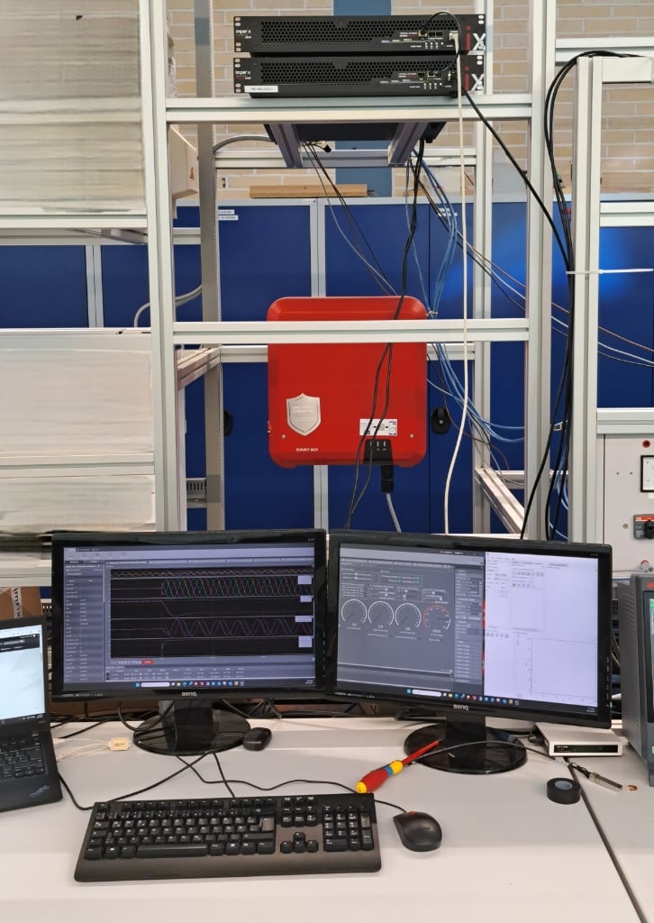
The setup (see Fig. 5) used to validate the proposed ANN-based control of the output current of the converter includes the following imperix products:
- TPI8032, 22kW all-in-one programmable inverter
- ACG SDK toolbox for automated generation of the controller code from Simulink
and additional components :
- 1x DC power supply
- Three-phase grid connection or three-phase power amplifier
Downloads
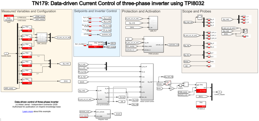
The full Simulink model, as shown in Fig. 6, with a trained neural network whose parameters are saved as nn_parameters.mat, is available for download using the link below:
Experimental results
To experimentally validate the performance of the FNN-based controller, it is implemented side-by-side with the vector current controller in the Simulink model, as shown in Fig. 7.
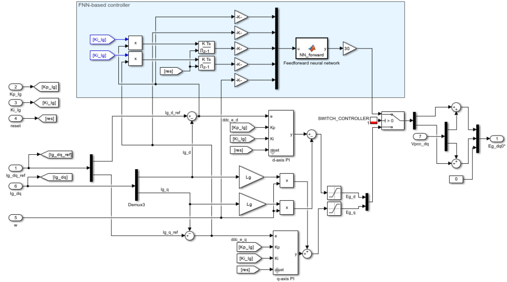
Fig. 7: FNN-based controller implementation in Simulink
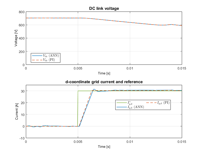
The experimental performance of the TPI8032 was evaluated at a switching and control frequency of 20 kHz with a line-to-neutral grid voltage of 230 V at the point of common coupling (PCC). To assess control robustness, a dynamic test scenario was configured in which the DC link voltage is programmed to drop from approximately 700 V to 600 V, right after the application of a step-input of 30A in the d-axis current reference. This DC link voltage drop, therefore, coincides with a step change in the d-axis output current reference () from 0 A to 30 A at t =5ms.
As illustrated in the results shown in Fig. 8, the FNN-based controller demonstrates a tracking performance similar to a PI controller. Despite the varying DC link voltage, a dynamic condition that was notably excluded from the training dataset, the FNN response (blue trace) closely tracks the reference and exhibits a transient response that nearly replicates the conventional PI-based vector current control scheme (dashed orange trace). This confirms that the FNN has successfully generalized its learning to respond to unseen operating conditions. Furthermore, the implementation proves to be computationally efficient; the execution of the FNN algorithm on the B-Board PRO embedded platform of TPI8032 consumes between 35% and 45% of the available cycle time at 20 kHz, ensuring the computational load remains well within the CPU’s capacity limits.
Conclusion
The example implementation demonstrates that a shallow ANN can effectively emulate the mapping of a discrete PI current controller in a grid-following converter while maintaining the deterministic, low-latency execution required for a real-time embedded target. However, the success of the approach is strictly dependent on the quality and breadth of the training dataset. While the ANN-based controller showed an ability to generalize to conditions like varying DC-link voltages not explicitly included in training, insufficient data coverage or limited training time remains a primary factor that can lead to subpar performance during unexpected transients. Rigorous cross-validation and the implementation of auxiliary safety mechanisms are essential to mitigate the risk of instability. Contrary to the assumption that ANN requires heavy computing power, this implementation proves that shallow ANNs can be effective and sufficient for power electronics control applications.
References
[1] M. R. G. Meireles, P. E. M. Almeida and M. G. Simoes, “A comprehensive review for industrial applicability of artificial neural networks,” in IEEE Transactions on Industrial Electronics, vol. 50, no. 3, pp. 585-601, June 2003.
[2] S. Zhao, F. Blaabjerg and H. Wang, “An Overview of Artificial Intelligence Applications for Power Electronics,” in IEEE Transactions on Power Electronics, April 2021.
[3] B. K. Bose, “Neural Network Applications in Power Electronics and Motor Drives—An Introduction and Perspective,” in IEEE Transactions on Industrial Electronics, Feb. 2007.
[4] S. Brunton, and J. Nathan Kutz, “Data-driven science and engineering: Machine learning, dynamical systems, and control“, Cambridge University Press, 2022.
To go further from here…
More information on the control of TPI8032 as a grid-forming inverter can be found in TN167. The following are some of the other notes that can be useful:
PN190: Getting started with th TPI8032
TN166: Active front end (AFE)