Cascaded H-bridge converter control

Table of Contents

This article focuses on the control of a star-connected cascaded H-bridge (CHB) using voltage balancing controllers superimposed on a state-of-the-art cascaded voltage regulator with an inner current control loop.

Typical applications for a modular topology using star-connected cascaded H-bridges are solid-state transformers (see AN015) and static synchronous compensators (STATCOM, see AN013) introduced in [1]. STATCOMs are widely used in power distribution and industry to actively control the reactive power flow and thus stabilize the grid voltage. In [1], it is noted that the main control challenge is to keep the capacitor voltages balanced.

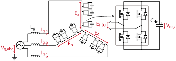
The topology of the star-connected cascaded H-bridge is presented below (Figure 1), followed by the description of the main controller and the balancing controllers. Finally, experimental results are shown, using imperix power modules and the B-Box RCP programmed with ACG SDK on Simulink or PLECS .

Schematic of the cascaded H-bridge converter — Figure 1: Schematic of the star-connected cascaded H-bridge STATCOM with N H-bridge submodules (N/3 per phase branch)

Control design of the cascaded H-bridge converter

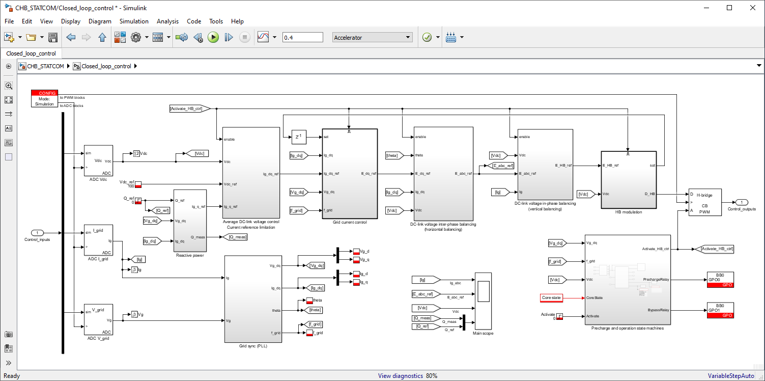
The overall control structure is depicted in Figure 2.

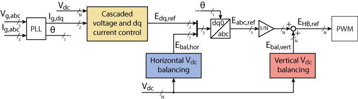
Overall control structure for the cascaded H-bridge converter — Figure 2: Overall control structure for the cascaded H-bridge

As proposed in [2], the structure of the capacitor voltage balancing strategy distinguishes between vertical balancing (across the submodules within a branch) and horizontal balancing (across the 3 branches of the whole converter). The functionalities of each control block are described in the following paragraphs.

Grid synchronization (PLL)

The dq reference frame is synchronized to the grid frequency and aligned with the phase voltage $V_{g, a}$. This is implemented in the PLL block proposed in Synchronous reference frame (SRF) PLL (TN103).

Cascaded voltage and dq current control

The principle of cascaded voltage control is detailed in Cascaded voltage control (TN108) for the case of a DC/DC converter. The same idea can be used for a grid-connected cascaded half-bridge topology, with the following adaptations:

The current responsible for a change in DC-link voltage is the d-current obtained by dq transformation of the grid currents. Thus, the inner current control loop is implemented as the dq controller described in vector current control (TN106). This structure also allows controlling the q-current, whose reference is computed to meet the reactive power demand.
The bandwidth of the voltage controller must be limited to the grid frequency. This way, the d-current reference Ig_d_ref only contains harmonics below the grid frequency, which ensures a low distortion of the grid currents.
The d-current is a scalar value that can only influence the total energy stored in the capacitors. As proposed in [2], the controlled voltage is then the average of all capacitor voltages. The individual capacitor voltages are in turn only regulated with so-called vertical and horizontal balancing controllers.

The structure of the cascaded voltage and dq current controller is shown in Figure 3. The details on the implementation of the individual blocks are given hereafter.

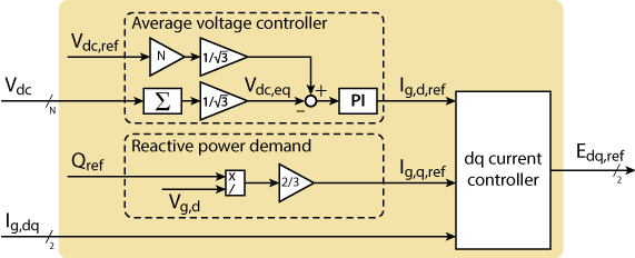
Figure 3: Structure of the cascaded voltage and dq current control for the grid-connected cascaded H-bridge

Reactive power demand (q current reference)

In the case of STATCOMs, the main control objective is the tracking of a reactive power reference. When the dq reference frame is aligned with the grid voltage Vg_a, the reactive power is simply obtained as [1]

$$Q = \frac{3}{2}\cdot V_{g,d}\cdot I_{g,q}.$$

The q-current reference $I_{g,q,\text{ref}}$ is then computed as

$$I_{g,q,\text{ref}}=\frac{2}{3}\cdot\frac{Q_\text{ref}}{V_{g,d}},$$

where $Q_\text{ref}$ is the reactive power demand.

Average voltage controller (d current reference)

The design of the average capacitor voltage controller relies on the equivalent average voltage and capacitance, where $N$ is the total number of H-bridge modules:

$$V_{dc,eq} = \frac{1}{\sqrt{3}}\cdot\sum_{i=0}^{N-1}V_{dc,i}$$

$$C_{dc,eq} = 3\cdot\frac{C_{dc}}{N}.$$

These quantities represent the energy-equivalent DC-link voltage and capacitance of a non-cascaded 3-phase inverter, as in vector current control (TN106).

The transfer function of the plant can be expressed using the equivalent DC-link voltage and capacitance [3]:

$$G_{plant}(s) = \frac{1}{1+s\cdot T_{cc}}\cdot \frac{1}{s\cdot C_{dc,eq}}\cdot\frac{3}{2}\cdot\frac{V_{g,d}}{V_{dc,eq}},$$

where $T_{cc}$ is the equivalent first-order time constant of the inner current control loop.

The controller is designed as a PI controller of the form:

$$G_{PI}(s) = K_{p,V}+\frac{K_{i,V}}{s}.$$

The open loop transfer function $G_{ol}(s) = G_{plant}(s)\cdot G_{PI}(s)$ is shaped according to the criteria:

the bandwidth is $\omega_{BW}$: $$\left| G_{ol}\left(j\omega_{BW}\right)\right| = 1$$
the phase margin is $\phi_{PM}$: $$\text{arg}\left(G_{ol}\left(j\omega_{BW}\right)\right) = -180° +\phi_{PM}.$$

It can be assumed that the bandwidth $\omega_{BW}$ is much smaller than the bandwidth of the inner control loop $1 / T_{cc}$. Therefore, the factor $1/(1+s\cdot T_{cc})$ can be neglected at $s = j\omega_{BW}$. The solution of the two equations above can then be expressed in terms of $K_{p, V}$ and $K_{i, V}$.

The gains of the PI controller are computed as:

$$K_{p,V} = \omega_{BW}\cdot\frac{2}{3}\cdot \frac{V_{dc,eq}}{V_{g,d}} \cdot C_{dc,eq}\cdot \sqrt{\frac{\text{tan}^2(\phi_{PM})}{1+\text{tan}^2(\phi_{PM})}}$$

$$K_{i,V} = K_{p,V}\cdot\frac{\omega_{BW}}{\text{tan}(\phi_{PM})}.$$

By choosing the bandwidth as $\omega_{BW} = 0.8\cdot\pi\cdot f_{grid}$ and the phase margin as $\phi_{PM} = 50°$, a good compromise between tracking dynamics and damping is obtained in simulation and experimentally.

dq current controller

The dq current controller is implemented as proposed in vector current control (TN106). Note that the only difference with the present article is the convention used for the sign of the grid currents (positive when injected into the grid). The sign of the currents Ig_abc and Ig_dq must therefore be inverted in all equations and block diagrams.

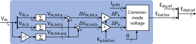
Horizontal voltage balancing

An imbalance of the average capacitor voltages across the three branches is equivalent to an imbalance of the stored energy in the branches. Consequently, such an imbalance can be compensated by acting on the active power flow into each one of the branches. In [2], it is shown that asymmetric branch power flows can be achieved by applying an appropriate common-mode voltage (corresponding to a star-point potential) oscillating at the grid frequency. This balancing common-mode voltage can be calculated as below, using $\alpha_2 = \frac{1}{2} I_{g,d}$, $\alpha_3 = \frac{1}{2} I_{g,q}$, $\beta_2 = -\frac{1}{4} I_{g,d} + \frac{\sqrt 3}{4} I_{g,q}$ and $\beta_3 = -\frac{\sqrt 3}{4} I_{g,d} \ – \frac{1}{4} I_{g,q}$.

The computations in [2] are based on the positive-negative-zero sequence representation, but the same approach can be used using the dq grid currents and branch voltages. The common mode voltage is modeled by its amplitude $V_{cm}$ and phase $\phi_{cm}$:

$I_{g,a}(t) = I_{g,d}\cdot\text{cos}(\omega t)\ – I_{g,q}\cdot\text{sin}(\omega t)$

$I_{g,b}(t) = I_{g,d}\cdot\text{cos}(\omega t-\frac{2\pi}{3})\ – I_{g,q}\cdot\text{sin}(\omega t-\frac{2\pi}{3})$

$I_{g,c}(t) = I_{g,d}\cdot\text{cos}(\omega t+\frac{2\pi}{3})\ – I_{g,q}\cdot\text{sin}(\omega t+\frac{2\pi}{3})$

and

$E_{a}(t) = E_{d}\cdot\text{cos}(\omega t)\ – E_{q}\cdot\text{sin}(\omega t) + V_{cm}\cdot\text{cos}(\omega t+\phi_{cm})$

$E_{b}(t) = E_{d}\cdot\text{cos}(\omega t-\frac{2\pi}{3})\ – E_{q}\cdot\text{sin}(\omega t-\frac{2\pi}{3}) + V_{cm}\cdot\text{cos}(\omega t+\phi_{cm})$

$E_{c}(t) = E_{d}\cdot\text{cos}(\omega t+\frac{2\pi}{3})\ – E_{q}\cdot\text{sin}(\omega t+\frac{2\pi}{3}) + V_{cm}\cdot\text{cos}(\omega t+\phi_{cm}).$

The active power flowing into each branch is obtained by multiplying the grid current with the corresponding branch voltage and then ignoring the oscillating terms:

$P_{br,a} = \frac{1}{2} E_{d}\cdot I_{g,d} + \frac{1}{2} V_{cm}\cdot I_{g,d}\cdot\text{cos}(\phi_{cm}) + \frac{1}{2} V_{cm}\cdot I_{g,q}\cdot\text{sin}( \phi_{cm})$

$P_{br,b} = \frac{1}{2} E_{d}\cdot I_{g,d} + \frac{1}{2} V_{cm}\cdot I_{g,d}\cdot\text{cos}(\phi_{cm}+\frac{2\pi}{3}) + \frac{1}{2} V_{cm}\cdot I_{g,q}\cdot\text{sin}(\phi_{cm}+\frac{2\pi}{3})$

$P_{br,c} = \frac{1}{2} E_{d}\cdot I_{g,d} + \frac{1}{2} V_{cm}\cdot I_{g,d}\cdot\text{cos}(\phi_{cm}-\frac{2\pi}{3}) + \frac{1}{2} V_{cm}\cdot I_{g,q}\cdot\text{sin}(\phi_{cm}-\frac{2\pi}{3}).$

Using the total active power

$P_{tot} = \frac{3}{2} E_{d}\cdot I_{g,d}$

and the definitions of $\alpha_2$, $\alpha_3$, $\beta_2$, and $\beta_3$ above, the power asymmetry in branches a and b can be found as:

$\Delta P_a = P_{br,a} \ – \frac{1}{3} P_{tot} = \alpha_2\cdot V_{cm}\cdot\text{cos}(\phi_{cm}) + \alpha_3\cdot V_{cm}\cdot\text{sin}(\phi_{cm})$

$\Delta P_b = P_{br,b} \ – \frac{1}{3} P_{tot} = \beta_2\cdot V_{cm}\cdot\text{cos}(\phi_{cm}+\frac{2\pi}{3}) + \beta_3\cdot V_{cm}\cdot\text{sin}(\phi_{cm}+\frac{2\pi}{3}).$

Since all 3 power asymmetries sum up to 0, the power asymmetry in branch c does not form an independent equation and is therefore not needed.

Solving these two equations in terms of $V_{cm}$ and $\phi_{cm}$ allows finding the amplitude and phase of the common-mode voltage which is necessary to achieve the desired branch power asymmetries $\Delta P_a$ and $\Delta P_b$ [2]:

$$\phi_{cm} = \text{atan}\left(\frac{- \Delta P_b \cdot \alpha_2 + \Delta P_a\cdot\beta_2 }{\Delta P_b\cdot\alpha_3-\Delta P_a\cdot\beta_3}\right)$$

$$V_{cm} = \frac{\Delta P_a}{\alpha_2\cdot\text{cos}(\phi_{cm})+\alpha_3\cdot\text{sin}(\phi_{cm})}.$$

Using properties of the trigonometric functions, the expression for the resulting balancing voltage signal $E_{bal, hor} = V_{cm}\cdot \text{cos}(\omega t + \phi_{cm})$ simplifies to the expression below.

The balancing voltage is computed as:

$$ E_{bal,hor} = \frac{(\Delta P_a\cdot\beta_3-\Delta P_b\cdot\alpha_3)\cdot\text{cos}(\omega t)+(\Delta P_a\cdot\beta_2-\Delta P_b\cdot\alpha_2)\cdot\text{sin}(\omega t)}{\alpha_2\cdot\beta_3-\alpha_3\cdot\beta_2}.$$

The proposed balancing controller is a simple proportional controller that takes the voltage imbalances as input and outputs the branch power asymmetries $\Delta P_a$ and $\Delta P_b$. Thanks to the purely integral nature of the plant (capacitor), the proportional controller yields no steady-state error.

The required common-mode voltage $E_{bal, hor}$ can then be computed from the equations above and is appended as 0-component to the voltage reference E_dq_ref. The whole control structure of the horizontal voltage balancing is illustrated in Figure 4.

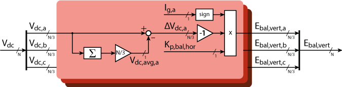
Structure of the horizontal voltage balancing controller for cascaded H-bridge — Figure 4: Structure of the horizontal voltage balancing controller

Vertical voltage balancing

For the sake of readability, this paragraph will only focus on the vertical voltage balancing within a branch of the cascaded h-bridge. The same procedure is implemented in branches b and c as well.

The voltage reference $E_{a,\text{ref}}$ must be distributed to the individual H-bridge submodules. The degree of freedom in the distribution of the voltage references can be used to adjust the individual power flowing into each H-bridge. This, in turn, allows the proper balancing of the energy content (i.e. capacitor voltage) of the H-bridges.

In [1], a simple distribution consisting of an evenly distributed term and an additive balancing term is proposed:

$$E_{HB,i_a,\text{ref}} = \frac{3}{N} E_{a,\text{ref}} + E_{bal,i_a},$$

where $\frac{N}{3}$ is the number of H-bridge submodules per branch. The balancing term $E_{bal,i_a}$ is the output of a proportional controller (gain $K_{p,bal,vert}$) taking the voltage imbalance $\Delta V_{dc,i_a}$ as error input:

$$ E_{bal, i_a} = \ – K_{p,bal,vert}\cdot\text{sign}(I_{g,a})\cdot \underbrace{\left(V_{dc,i_a}\ – \frac{3}{N}\sum_{i_a=0}^{\frac{N}{3}-1}V_{dc,i_a}\right)}_{\displaystyle \Delta V_{dc,i_a}}.$$

The structure of this concept is illustrated in the figure below.

Structure of the vertical voltage balancing controller for cascaded H-bridge — Figure 5: Structure of the vertical voltage balancing controller

The choice of $E_{\text{bal},i_a}$ ensures that the total branch voltage reference does indeed equal to $E_{a,\text{ref}}$:

$$\sum_{i_a=0}^{\frac{N}{3}-1} E_{HB,i_a} = \sum_{i_a=0}^{\frac{N}{3}-1} \left(\frac{3}{N} E_{a,\text{ref}} + E_{\text{bal},i_a}\right)$$ $$ = E_{a,\text{ref}} \ – K_{p,\text{bal},vert}\cdot\text{sign}(I_{g,a})\cdot\underbrace{\left(\sum_{i_a=0}^{\frac{N}{3}-1}V_{dc,i_a} – \frac{N}{3}\cdot\frac{3}{N}\cdot\sum_{i_a=0}^{\frac{N}{3}-1}V_{dc,i_a}\right)}_{=\ 0} = E_{a,\text{ref}}.$$

Moreover, to show that the chosen balancing voltage reference does indeed balance the capacitor voltages, the power flowing into the half-bridges (i.e. into the capacitors) must be analyzed.

Assuming that $E_{a}\approx E_{a,\text{ref}}$, the instantaneous power flowing into H-bridge $i_a$ can be expressed as:

$$ P_{i_a} (t)=I_{g,a}\cdot E_{HB,i_a} = I_{g,a}\cdot \frac{3}{N} E_a + I_{g,a}\cdot E_{\text{bal},i_a}. $$

Identically, the total instantaneous power flowing into the branch is

$$P_{tot,a}(t) = I_{g,a} \cdot E_a.$$

Consequently, the power asymmetry flowing into H-bridge $i_a$ is expressed as:

$$\Delta P_{i_a} = P_{i_a}\ – \frac{3}{N} P_{tot,a} = I_{g,a}\cdot E_{\text{bal},i_a}.$$

It appears that the power asymmetry $\Delta P_{i_a}$ and the voltage imbalance $\Delta V_{dc,i_a}$ are of opposite signs:

$$\Delta P_{i_a} =\ – K_{p,\text{bal},vert}\cdot\left|I_{g,a}\right|\cdot \Delta V_{dc,i_a}.$$

This shows that an H-bridge whose voltage is higher than the average will always receive less power than the average (and vice-versa). The choice proposed in [1] then indeed balances the capacitor voltages in the considered branch.

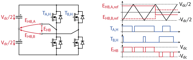
PWM modulation

In the proposed implementation, carrier-based PWM is used. The voltage reference for an H-bridge is split between the two half-bridges A and B:

$$E_{HB,A,\text{ref}} = \frac{1}{2}\cdot E_{HB,\text{ref}}$$

$$E_{HB,B,\text{ref}} = -\frac{1}{2}\cdot E_{HB,\text{ref}}.$$

To generate the gate signals, the resulting half-bridge reference voltages are compared to a common triangular carrier in the range $[-\frac{V_{dc}}{2}, \frac{V_{dc}}{2}]$, as shown in Figure 6.

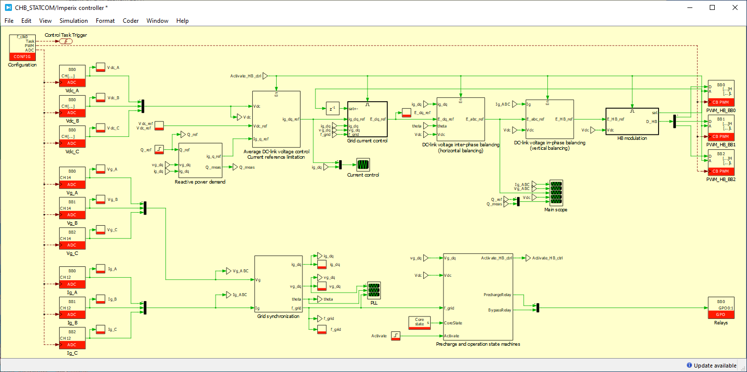
Figure 6: Illustration of the carrier-based PWM for H-bridges

Control software implementation

Two sets of files are proposed, suitable for implementing the control and simulating its behavior in MATLAB Simulink or Plexim PLECS environment.

Download TN165_CHB_control_Simulink.zip

Simulink model to control a cascaded H-bridge

Download TN165_CHB_control_PLECS.zip

PLECS model to control a cascaded H-bridge

The provided models allow the configuration of the number of H-bridges between 1 per phase (N=3) and 8 per phase (N=24). By default, 4 H-bridges per phase are configured (N=12) which allows wiring the cascaded H-bridge using the standard MMC bundle.

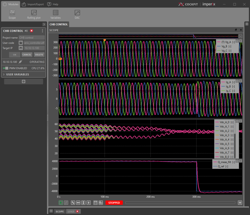
Experimental results

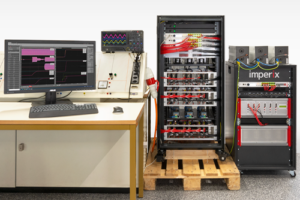
The control algorithm can be easily compiled using the ACG SDK and tested on imperix hardware. For instance, the standard MMC bundle allows connecting a total of N=12 H-bridges with little re-wiring effort and without additional hardware. Thanks to optical expansion boards for additional PWM output signals, the MMC bundle can be extended to control up to N=24 H-bridges. The resulting waveforms are monitored with the imperix Cockpit software and are visible in Figure 7. At t = 100 ms, the vertical balancing is activated, which forces the capacitor voltages to converge within each phase. At t = 200 ms, the horizontal balancing is activated, which forces all capacitor voltages to converge across the whole converter. At t = 300 ms, the reactive power reference is changed from 4 kVar to -4 kVAr.

Control of a cascaded H-bridge converter with monitoring in Cockpit software. — Figure 7: Experimental results for the grid-connected cascaded H-bridge with N=24 H-bridges showing the effect of balancing and a reactive power step response

Academic references

[1] H. Akagi, S. Inoue, and T. Yoshii, “Control and Performance of a Transformerless Cascade PWM STATCOM With Star Configuration,” in IEEE Transactions on Industry Applications, 43(4):1041–1049, July-Aug. 2007.

[2] M. Vasiladiotis, “Modular Multilevel Converters with Integrated Split Battery Energy Storage,” Ph.D. dissertation, EPFL, 2014

[3] C. Bajracharya, “Control of VSC-HVDC for wind power,” NTNU, 2008