Sampling techniques for power electronics

Introduction

Power electronic converters pose a specific sampling challenge: the signals of interest (currents and voltages) are low-frequency components, but they are combined with a high-frequency PWM ripple. This page explains the particularities of sampling in power electronics. It reviews conventional sampling methods such as anti-aliasing filters and synchronous sampling, and highlights their limitations. Finally, it introduces an advanced technique recommended for imperix controllers, the synchronous averaging.

Background and motivation

In any PWM-based power converter, the main electrical quantities such as currents and voltages are never perfectly smooth. Instead, they can be viewed as a low-frequency average value, on top of which a high-frequency component appears due to the switching action of the power devices. This high-frequency component is commonly called ripple.

Removing this ripple would require large or expensive passive components, so in practice a non-negligible ripple is often accepted. In many applications, what really matters for control and monitoring is the average value of the signal, (for example a 50/60 Hz current in an AC grid), while the ripple is mostly an unwanted side effect. The challenge is therefore to measure and control the average value even when a ripple is present.

Conventional sampling techniques

To tackle the above-mentioned challenge, two distinct techniques are commonly used: anti-aliasing low-pass filtering and synchronous sampling. Each provides an alternative way to reduce the influence of high-frequency ripple on the average measurement. The next sections present them.

1. Anti-aliasing low-pass filtering

A straightforward way to extract a low-frequency component (i.e. the average value) from a disturbed signal is to apply a low-pass filter. Choosing a sufficiently low cutoff frequency attenuates the ripple introduced by the PWMs. The controller can then sample the filtered signal and use it without strict synchronization with the PWM.

Anti-aliasing principle

Aliasing occurs when the signal fed to the sampler (ADC) still contains frequency components above \(f_s/2\). In that case, the Shannon–Nyquist requirement is violated and the out-of-band content is folded back into the baseband as false low-frequency components [1], which distorts the measurement.

Fig. 2 illustrates aliasing for a signal containing a component above \(f_s/2\). As the Shannon–Nyquist condition is not satisfied, that high-frequency component folds back into the low-frequency band and appears as a spurious lower-frequency term in the sampled signal.

The following Fig. 3 illustrates this effect on a simple example: a current ripple at 5 kHz is sampled at 6 kHz. In the reconstructed signal, this leads to an apparent frequency \(f_{alias​}= |f_{sampling​}−f_{signal​}| = 1 kHz\), even though the switching-averaged value remains constant (DC). This 1 kHz component is therefore not a physical low-frequency behaviour of the system, but a pure aliasing artefact introduced by the sampling process.

The role of an anti-aliasing low-pass filter is therefore to strongly attenuate all components with frequencies higher than \(f_s/2\) before sampling, so that their folded copies do not corrupt the useful low-frequency content.

Filter design trade-offs

The theoretical ideal low-pass filter is the “brick-wall” filter (Eq. 1). It perfectly passes the band of interest with zero phase shift and completely rejects higher-frequency components, thereby preventing aliasing without adding delay to the signal of interest.

$$ (1) \quad \quad
\frac{I_{\text{LPF ideal}}(j\omega)}{I(j\omega)} =
\begin{cases}
1 \angle 0 & \text{for } \omega < \omega_s/2 \\[4pt]
0 & \text{for } \omega \ge \omega_s/2
\end{cases}
$$

However, such an ideal, brick-wall filter cannot be implemented in practice, since it would be non-causal. In reality, a compromise must be found between bandwidth, group delay and attenuation. This compromise is entirely application-dependent and is determined by the amount of residual ripple that can be tolerated by the control system. To illustrate this trade-off, Fig. 4 shows the frequency response of a fifth-order Bessel low-pass filter for different bandwidths.

Reducing the cut-off frequency improves attenuation of the switching ripple, but it also increases the group delay. Using higher-order filters further sharpens the transition between passband and stopband and thus enhances ripple rejection for a given cut-off frequency, at the price of additional phase shift. In Fig. 4, a reasonable trade-off would be to set \(f_{Bandwidth} \simeq 0.2 f_{\mathrm{PWM}}\)

Once the filter parameters are chosen appropriately, the output waveform becomes essentially smooth. Therefore, the sampling instant doesn’t need to be controlled precisely.

To conclude, purely analog anti-aliasing filters remain attractive in situations where ADC sampling cannot be synchronized with the PWM. However, from a control perspective, the extra delay introduced by the low-pass filter directly degrades the achievable dynamic performance. Finally, when sampling can instead be time-aligned with the modulation, the anti-aliasing filter is generally sub-optimal compared with the techniques presented in the following sections, which explicitly exploit the deterministic and periodic nature of the ripple.

2. Synchronous sampling

In PWM converters, synchronous sampling is the most commonly used method to capture a value representative of the average current/voltage over a switching period [2]. The basic idea is to sample the waveforms at exactly the same frequency as the modulation, with a well-defined phase relationship.

At first glance, sampling at the switching frequency contradicts Shannon’s sampling theorem. However, when the sampling frequency is exactly equal to the ripple frequency, the corresponding alias appears at \(|f_\text{sample} – f_\text{ripple}| = 0 \text{Hz}\), then the folded component becomes a constant term due to aliasing.

With an appropriate sampling phase exactly at the middle of the PWM period (assuming a perfectly triangular ripple), the measured value normally coincides with the average value over one switching period and the folded component cancels out.

This approach is particularly attractive because it introduces essentially no additional sampling delay, unlike analog anti-aliasing filters whose attenuation is intrinsically linked to phase lag. As a result, synchronous sampling allows a higher control bandwidth [3]. On the other hand, this sampling method is also more sensitive to waveform distortions and non-idealities, as discussed in the following sections.

Limitations of synchronous sampling

Synchronous sampling is only valid as long as the captured waveform crosses its average value exactly at the chosen sampling instant. In practice, this condition is not always fulfilled, and significant deviations may occur. Three typical phenomena can induce such deviations and are discussed in the following sections.

Sensor bandwidth

One of the most common issues with synchronous sampling is the finite bandwidth of the sensors and the associated delay. In a triangular carrier, the current ripple equals its average value when the carrier reaches its peak or its valley. However, when the measurement chain introduces a non-negligible delay, the sampling phase must be shifted accordingly. If it is not, the controller samples the signal too early relative to the actual measured waveform.

Fig. 9 illustrates this effect for two current sensors with different bandwidths measuring the same signal. The cyan trace corresponds to a high-bandwidth sensor (\(f_B = 200f_{PWM}\)), while the green trace shows a low-bandwidth sensor (\(f_B = 7.5f_{PWM}\)). Without adjustment of the sampling instant, the low-bandwidth sensor may be sampled at a ripple phase that is not representative of the average value, resulting in a biased current measurement.

Non-linear ripple segment

One of the key assumptions behind synchronous sampling is that the ripple has a triangular shape. This requires the relevant transient time constant of the system, \(\tau\), to be much larger than the switching period, \(T_{sw}\)​. $$(3) \quad \quad T_{sw} << \tau \quad with \quad \tau = \frac{L}{R}$$
Where \(L\) and \(R\) denote the equivalent inductance and resistance seen by the converter, typically comprising the output filter and the load. When Eq. 3 is not satisfied, the waveform can deviate significantly from a triangular shape, so that the chosen sampling instant no longer corresponds to the true average value as illustrated in Fig. 10 and 11.

Thanks to the oversampling capability and waveform visualization available in Cockpit, this effect can be directly observed. In that case​, where the ripple departs significantly from a linear shape (where \(\tau\) is not much larger than \(T_{sw}\)), it is generally advisable to avoid synchronous sampling.

Switching-induced waveform distortion

With synchronous sampling, the current is measured at a single instant within each switching period. If noise or distortion (e.g. ringing effect) is present at that instant, the corresponding sample, and thus the inferred average waveform, is directly affected. This situation is particularly critical when sampling close to a switching transition, since the ripple is often strongly disturbed at that moment. As a result, synchronous sampling tends to be more sensitive to measurement errors at high switching frequencies or with high-to-extreme modulation depths, as shown in Fig. 12 and 13.

As can be observed in Fig. 13, at large modulation depths the ADC sampling instant can occasionally fall on (or very close to) a switching transition. In that case, the measured sample is contaminated by the switching-related disturbance (e.g., ringing), and this error is then propagated to the reconstructed waveform, recreating artificial spikes (Fig. 12).

It should also be noted that, in Fig. 12, the slight deviation of the cyan waveform (synchronous sampling) with respect to the yellow waveform (synchronous averaging) is mainly caused by a non-linear ripple and therefore cannot be directly attributed to sampling on a switching event.

Synchronous averaging

Thanks to oversampling, i.e. sampling the current faster than the control update rate, it is possible to estimate the average ripple value without relying on a single sampling instant. The average is computed over a time window chosen to span one switching period. The result is an approximation of the true period-average, and its accuracy improves as the oversampling ratio increases.

Fig. 14 illustrates the difference with synchronous sampling: both methods provide the average over one period of CLK0. From a control perspective, the synchronous averaging results in an additional group delay of half a switching period in the measurements.

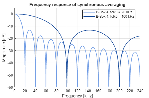
Fig. 15 shows the frequency response of synchronous averaging on a B-Box 4 (20 MHz sampling) for two different control frequencies. The notches appear exactly at \(f_{\text{clk0}}\)​ and at its harmonics, which means that the switching ripple is strongly rejected while the average value is preserved.

An important consequence of this approach is that the resulting average value is independent of the sampling phase (i.e. all samples are equally weighted). The averaging window can therefore be placed anywhere within the PWM period, in particular, as late as possible before the duty-cycle update instant. This often compensates for part of the additional delay introduced by synchronous averaging, depending on the computation time.

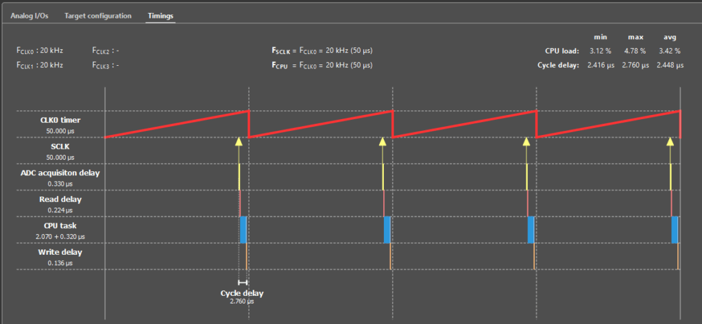
This point is illustrated in Fig. 16, where the synchronous averaging window is positioned with respect to the CPU load. Using a buck converter example and a B-Box 4, the extra delay attributable to synchronous averaging is approximately 3 µs over a 50 µs period, which is roughly 6% more than the minimum total loop delay.

A final benefit of synchronous averaging over synchronous sampling is the gain in effective resolution as the oversampling ratio increases (number of samples per CLK0 period). As with any digital low-pass filtering, averaging M uncorrelated samples increases the effective resolution by \(log_{2}(M)\) extra bits. Table 1 reports the effective resolutions obtained with synchronous averaging on imperix controllers.

Device CLOCK_0	B-Box 4 20 kHz	B-Box 4 100 kHz	B-Box RCP3.0 20 kHz	B-Box RCP3.0 100 kHz
# of averaged samples	1000	200	25	5
Effective resolution [bits]	26	23.6	20.6	18.3

Sampling recommendation using imperix controllers

Finally, Table 2 summarizes the recommended sampling techniques derived from experiments on imperix controllers, but not tied to any controller-specific feature. As the table indicates, synchronous averaging is generally the preferred choice for most applications.

	Anti-aliasing LPF	Synchronous sampling	Synchronous averaging
Non-triangular carrier
Non linear ripple
Maximize control bandwidth
Noisy measurement
PWM and sampling cannot be synchronized

References

[1] A. V. Oppenheim, R. W. Schafer and J. R. Buck, Discrete Time Signal Processing, 2nd
edition. Englewood Cliffs, NJ: Prentice-Hall, 1999.

[2] F. Briz, D. Díaz-Reigosa, M. W. Degner, P. García and J. M. Guerrero, “Current sampling and measurement in PWM operated AC drives and power converters,” The 2010 International Power Electronics Conference – ECCE ASIA, Sapporo, Japan, 2010, pp. 2753-2760.

[3] S. Buso and P. Mattavelli, “Digital control in power electronics,” Synthesis Lectures on Power Electronics, vol. 1, no. 1, pp. 1–158, 2006.