
Table of Contents
The System Identification (Sys. Id.) Injector block superimposes an excitation signal, such as a pseudorandom binary sequence (PRBS), on a scalar user-code signal. The resulting excitation is used to estimate the frequency response between two signals of the system under test. The block is the user-code component of the imperix System Identification toolbox:
- On imperix controllers, the experiment is configured and launched from the Cockpit System Identification module (PN306). The Scope module (PN301) records the data, from which Cockpit estimates and displays the frequency response.
- In Simulink or PLECS simulations, the block records the experiment and estimates the frequency response at the end of the simulation run.
This page focuses on configuring the injector block in Simulink/PLECS. PN215 (parametric identification of a buck converter) and PN216 (controller tuning in the frequency domain) present application examples.
Experiments with Cockpit’s System Identification module can be scripted using Python. A dedicated set of methods is available in the Python library.
Principles of operation
An identification experiment, whether executed on hardware or in simulation, runs in two phases:
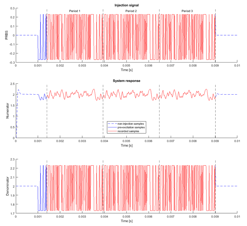
- Excitation and recording. The excitation is injected at the control task rate, and the numerator and denominator signals are recorded.
- Estimation. The recorded data is used to compute the frequency response from the denominator to the numerator signal. In most cases, the numerator is the output signal and the denominator is the input signal, but this is not always the case.
Excitation signal
The excitation \(p(t)\) is a pseudorandom binary sequence (PRBS), which is a deterministic, periodic binary signal whose spectrum resembles white noise. A single experiment therefore excites all frequencies at once. Each bit lasts one control period \(T_s\), so the sequence is clocked at the control task rate \(f_s = 1/T_s\).
The two binary levels of the PRBS sequence are separated by the peak-to-peak value \(A_\mathrm{pp}\).
Advanced PRBS settings. The order \(N\), the number of repetitions \(R\) and the pre-excitation time \(T_\mathrm{pre}\) set the duration and frequency resolution of the experiment. One PRBS period contains \(L\) samples:
\[ L = 2^N – 1 \]
The injected signal consists of a pre-excitation part of duration \(T_\mathrm{pre}\), followed by \(R\) complete periods. The pre-excitation brings the system into the periodic steady state induced by the PRBS. The main part continues the same binary sequence. The total excitation duration is:
\[ T_\mathrm{PRBS} = T_\mathrm{pre} + L \cdot R \cdot T_s \]
The frequency response is obtained on the frequency grid defined by the PRBS period, from the resolution \(\Delta f\) up to the Nyquist frequency:
\[ f_k = \frac{k}{L\,T_s}, \qquad k = 1, \dots, \frac{L-1}{2}, \qquad \Delta f = \frac{f_s}{L} \]
For example, with the default settings (\(N = 12\), \(R = 10\), \(T_\mathrm{pre} = L \cdot T_s\)) and \(f_s = 50\,\mathrm{kHz}\): \(L = 4095\), \(\Delta f \approx 12.2\,\mathrm{Hz}\) and \(T_\mathrm{PRBS} \approx 0.90\,\mathrm{s}\). Higher order improves resolution at the cost of a longer experiment, and more repetitions reduce noise.
Injection modes
The block output depends on the injection mode, where \(p(t)\) is the excitation signal and \(\overline{in}\) is the average of the input signal over the last 10 ms before the injection starts:
\[ \mathrm{out}(t) = \begin{cases} \mathrm{in}(t) + p(t) & \text{closed-loop mode, during injection} \\ \overline{in} + p(t) & \text{open-loop mode, during injection} \\ \mathrm{in}(t) & \text{otherwise} \end{cases} \]
- Closed-loop mode keeps any control loop running through the injector active during the experiment.
- Open-loop mode opens any control loop running through the injector for the duration of the experiment. In this mode, the
openblock output is set to 1, which can be used to pause integrators upstream to prevent windup.
Both modes give identical results when the injector follows a constant signal, such as a reference. The open-loop mode should not be used when the opened loop is unstable, e.g. a loop containing an integrator.
Frequency response estimation
The frequency response is computed from the spectra of the numerator \(y\) and the denominator \(u\) at the excited frequencies.
With a PRBS excitation, the Empirical Transfer Function Estimate (ETFE) [1] is computed only from data recorded during the \(R\) complete periods; pre-excitation samples are discarded. The estimation proceeds in three steps:
- The recorded data is split into \(R\) segments of \(L\) samples, one per PRBS period.
- One ETFE is computed per segment \(r\) as the ratio of the Discrete Fourier Transforms (DFT) of the numerator and denominator.
- The final estimate is the average of the \(R\) estimates.
\[ \hat{G}_r(f_k) = \frac{Y_r(k)}{U_r(k)}, \qquad Y_r(k) = \sum_{n=0}^{L-1} y_r[n]\, e^{-j 2\pi k n / L} \]
\[ \hat{G}(f_k) = \frac{1}{R} \sum_{r=1}^{R} \hat{G}_r(f_k) \]
Each segment spans exactly one period of a periodic excitation. Therefore, no window is applied and no spectral leakage occurs, provided the system is in periodic steady state [2]. Averaging over \(R\) periods reduces the influence of uncorrelated noise. The estimate is valid only if the system behaves linearly around its operating point; saturation, including that of the Output safety limits, invalidates it.
Results and analysis
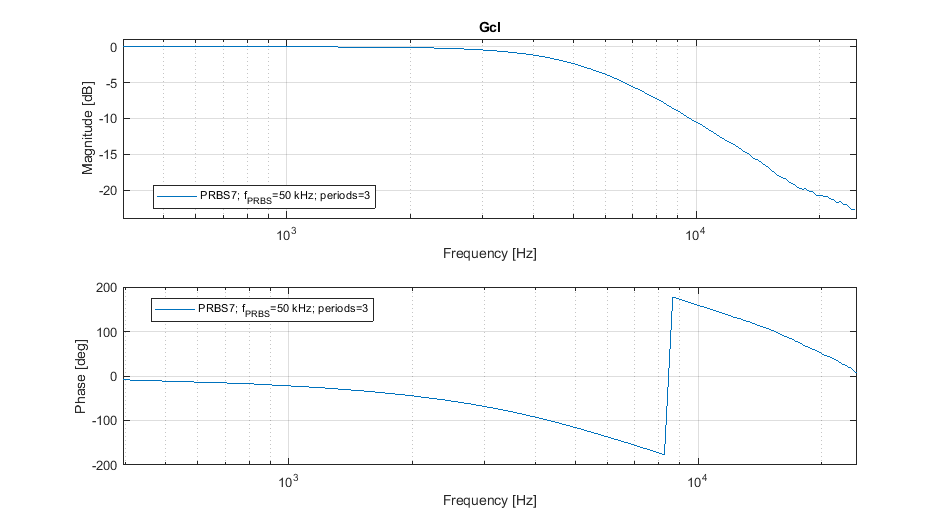
While the overall process executes identically on real hardware or in simulation, the software environment differs. The table below summarizes how the results are displayed:
| Environment | Estimation starts | Results |
|---|---|---|
| Cockpit | When the Scope acquisition ends | – Bode plot in Cockpit’s Sys. Id. module – Time-domain data in the Scope module. Snapshots and export options are available |
| Simulink | At the end of the simulation run | – Struct <injector name>_data in the MATLAB base workspace– Bode plot displayed automatically |
| PLECS | At the end of the simulation run | – system_response.csv auto-exported (time domain data) – etfe_result.csv auto-exported (frequency domain data)Both files are located in a folder named after the injector, next to the model file. |
Quick settings
With the default settings, the PRBS amplitude is the only parameter that must be chosen. All other parameters are advanced and can be left at their defaults for a first experiment. With an imperix controller, an experiment takes four steps:
- Insert the block on the signal to perturb, name it, and add Probe blocks on the numerator and denominator signals. Build and deploy the model.
- Bring the system to the intended operating point and wait for steady state.
- In the Cockpit Sys. Id. module, select the injector, set the Peak-to-peak amplitude, and select the numerator and denominator.
- Press Inject excitation. The Bode plot is displayed once the Scope acquisition is complete.
In simulation, steps 3 and 4 are replaced by enabling Simulate system identification in the block mask, connecting the num and den ports, and setting the amplitude.
Block parameters
Injector parameters
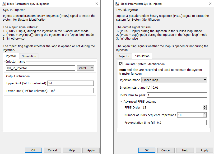
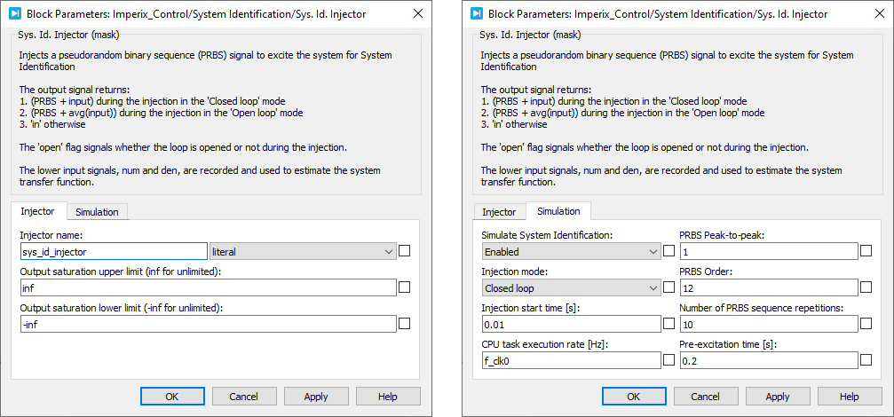
- Injector name: identifies the injector in the Cockpit Sys. Id. module and names the simulation outputs.
- Output safety limits: optionally saturate the block output. They are disabled by default and serve only as a protection: if they are reached, the excitation is distorted, and the estimate is invalid.
Simulation parameters
The simulation parameters are revealed when the Simulate System Identification option is selected in the Simulation parameters tab. When this option is active, the block records the input model data and estimates the frequency response at the end of the simulation.
For a given Injector name (e.g. sys_id_injector), Simulink saves the system identification data in a struct variable with that name and a suffix “_data” (e.g. sys_id_injector_data) in the MATLAB base workspace. PLECS, on the other hand, saves two CSV files (system_response.csv and etfe_result.csv) in a folder with the same name as the injector next to the PLECS model file.
The simulation parameters include:
- Injection mode: allows choosing between open-loop and closed-loop injection modes.
- Injection start time [s]: injection start time in the simulation; the system should be in steady state.
- PRBS peak-to-peak: configures the difference between the high and low state values of the pseudorandom binary sequence.
- Advanced PRBS settings:
- PRBS order: sets the PRBS period length. For an order \(N\), the period length is \(L=2^N-1\).
- Number of PRBS sequence repetitions: sets how many PRBS periods are injected. For \(R\) repetitions, the module estimates \(R\) frequency responses using recorded data. The module displays the final estimate, calculated as the average of these estimates.
- Pre-excitation time [s]: sets the duration before the \(R\) full periods. The data recorded over this interval is disregarded.
In PLECS, an additional parameter, CPU task execution rate [Hz], must be configured. For a CLK0 frequency \(F_{\text{CLK0}}\) and a postscaler value configured in the CONFIG block this parameter should be set to \(F_{\text{CPU}} = F_{\text{CLK0}}\) / postscaler.
Signal specification
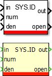
- in is the block input signal, upon which the PRBS is injected
- num and den inputs only appear if the Simulate system identification option is activated. They record the system’s response so that the transfer function can be estimated afterward.
- out is the main block output. Its value depends on the injection mode:
- PRBS + in, during injection in the closed-loop mode;
- PRBS + the estimated average of in, during injection in the open-loop mode;
- in, otherwise.
- The open signal is a binary signal designed to prevent integral windup in open-loop mode by pausing the error accumulation during the injection. This output produces:
- 1, during injection in the open-loop mode,
- 0, otherwise.
Masks
References
[1] Lennart Ljung, System Identification: Theory for the User, Pearson Education, 1998,
ISBN: 978-0-132-44053-0
[2] R. Pintelon and J. Schoukens, System Identification: A Frequency Domain Approach, 2nd ed. Hoboken, NJ, USA: Wiley-IEEE Press, 2012.
 By Andrea Lauri • September 14, 2026 • PN216
 By Mateja Ilić • September 14, 2026 • PN306