Controller tuning in the frequency domain

This note describes a simple frequency-domain PI controller tuning procedure using the imperix System Identification toolbox, available starting from imperix ACG SDK version 2026.3. The toolbox is a helpful companion in several relevant scenarios:

• It provides the system’s frequency response, allowing validation of an analytical model or helping the user derive one;
• It helps in assessing compliance with the chosen control objectives when tuning the controller, such as closed-loop stability margins or regulation performance.

This article considers a buck converter and describes the steps to tune the inductor current controller using the magnitude-optimum method, deriving all necessary parameters from system identification data and finally validating the design with the System Identification Toolbox.

Controller tuning procedure

The goal of this section is to tune the $k_i$ and $k_p$ gains of the PI controller starting from the frequency response of the plant $G(s)$. The following schematic shows the system under consideration:

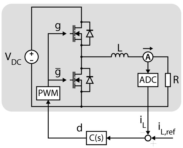
The plant $G(s)$ is the buck converter and includes the RL circuit, the power module, the sensors, and the PWM modulator (i.e., the system actuator). It corresponds to the grey area in the above schematic. The controller $C(s)$ to be designed is implemented in an imperix controller, and its structure is a typical parallel PI controller:

Conceptually, the above picture corresponds to the following control scheme:

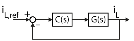
The transfer function of interest for the controller-tuning procedure is from the duty cycle $d$ to the inductor current $i_L$. Its frequency response is identified in PN215, and it is obtained from a system with the following parameter values:

Description	Symbol	Value
DC input voltage	$V_\mathrm{dc}$	200 V
Filter inductance	$L$	2.65 mH
Load resistance	$R$	11.9 Ω
Switching frequency	$F_\mathrm{sw}$	50 kHz

Derivation of necessary parameters

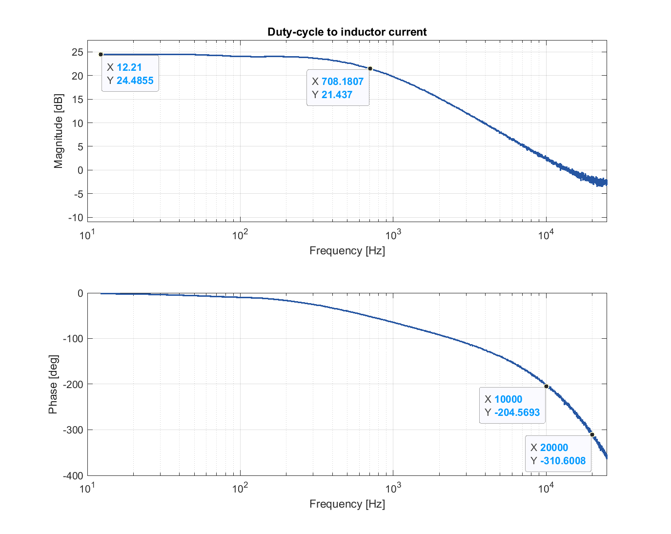
The following Bode plot shows the frequency response resulting from the procedure in PN215. By visual inspection, one notices the following characteristics:

• Flat response in the low-frequency domain;
• A roll-off of 20dB/dec in the high-frequency region;
• The typical phase profile of a system with a delay, where the phase lag increases linearly with the frequency.

Therefore, a first-order system plus delay is a good candidate to model the system behavior:

The magnitude-optimum controller tuning procedure requires the knowledge of $K$, $\omega_p$, and $T_d$ to derive the PI controller $k_i$ and $k_p$ gain values:

• $K$ corresponds to the static gain of the plant, that is $|G(0)|$. The value at the lowest available frequency is a good approximation of that.
• $\omega_p$ is the frequency of the system pole (in rad/s). For a first-order system like this, it is the frequency at which the plant’s magnitude is 3dB lower than $|G(0)|$.

Finally, one can estimate $T_d$ directly from the phase Bode plot, provided $\omega_p$ is sufficiently far below the high-frequency region. As the delay provides a phase lag that grows linearly with the frequency, the following relation holds:

where $\varphi$ is in radians, $\omega$ is in radians per second, and $T_d$ is in seconds. Using the values available in the graphs yields the following parameters:

It is also possible to compute the total delay $T_d$ directly as described in PN142. In such a system, the delay $T_d$ is inherent to the controller and includes the analog acquisition delay, the control-algorithm computation delay, and the PWM modulator delay. With a switching frequency of 50kHz and synchronous averaging in the analog acquisition, the resulting delay is $T_d=30\,\mathrm{\mu s}$, which is close to the value estimated above.

PI controller tuning

Once the required parameters are determined, the magnitude-optimum design procedure is straightforward for a first-order system with delay. It merely consists of computing the gains directly from the formulas:

TN105 describes the derivation of these formulas. The resulting values are $k_p \approx 0.23$ and $k_i \approx 1011.5$.

Experimental validation

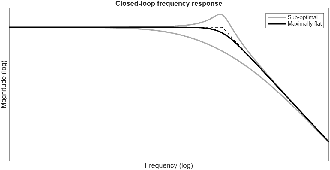
To validate the control design, it’s possible to identify the frequency response of the closed-loop transfer function from the inductor current reference to the measured inductor current. For a magnitude-optimal controller, the expected response is maximally flat up to a certain frequency range (the system bandwidth). If the designed controller is optimal, different $k_i$ or $k_p$ values should lead to an overdamped or underdamped response.

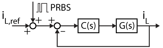
The procedure to obtain the system closed-loop transfer function consists of perturbing the inductor current reference signal and then computing the Empirical Transfer Function Estimation (ETFE) by taking the ratio of the Fourier transforms of the output signal (the perturbed inductor current) over the input signal (the perturbed current reference). In this case, i_Lref is perturbed, and it is measured together with i_L. The following schematic clarifies the idea. The System Identification toolbox handles the perturbation injection and transfer-function computation.

These Simulink and PLECS models are preconfigured to perform system identification on the closed-loop system. The Sys. Id. Injector block perturbs the system and then measures its response. The numerator signal is i_L, while the denominator is i_Lref.

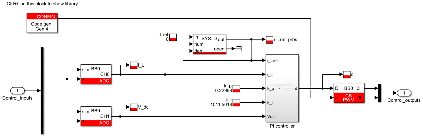
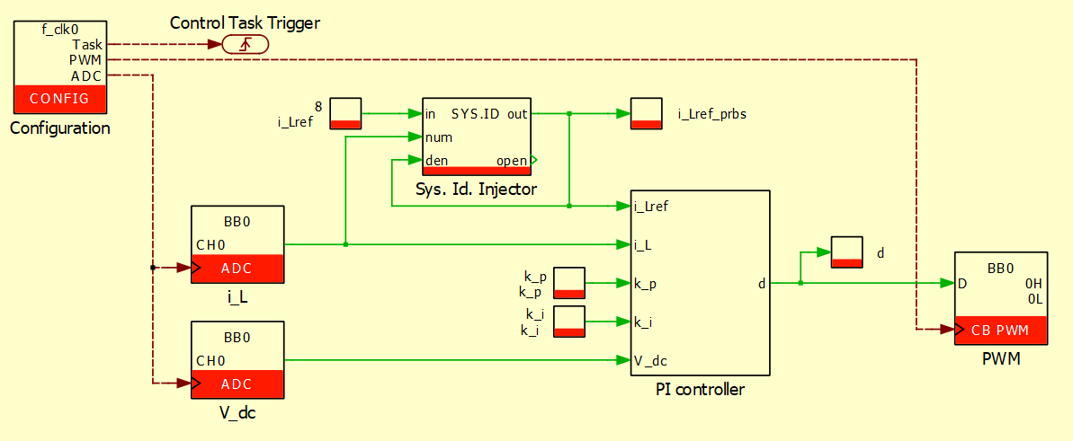
The models can be directly built and sent to an imperix controller by pressing Ctrl + B in Simulink or Ctrl + Alt + B in PLECS. More information on deploying the model to an imperix controller is available in PN138. After building the model, Cockpit should automatically open. The user can also open it manually. It will also automatically detect the Cockpit project file (.ixproj) provided with the models. This pre-configures the project workspace by adding a Scope module and a System Identification module, and adds the i_L, i_Lref, and d variables to the Scope.

Hardware setup description

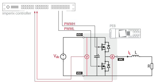
The following list describes the elements used to build the buck converter:

• A phase leg module (PEB-800-40, PEB8038, PEB8024, or PEB4050);
• A programmable controller (B-Box 4, B-Box 3, or B-Box 3 Micro);
• A DC power supply;
• An inductor and a resistor;

The following schematic conceptually illustrates the setup for the buck topology considered. The setup uses the phase leg module’s internal output current and input voltage sensors to measure $i_L$ and $V_\mathrm{dc}$.

Validation in Cockpit

Once Cockpit is open, it is possible to perform the identification by following these steps:

1. For best results, the system should operate at the same operating conditions as during characterization. This corresponds to an input DC voltage of 200 V and an average duty cycle of 0.5, as described in the parametric identification example in PN215.
2. Turn on the DC voltage source and make sure the variable V_dc settles around the expected value. If not, check the sensor’s sensitivity and whether it is connected to the correct channel. The PWM enable switch should be off, so i_L should be zero.
3. The tunable reference signals should bring the system to the desired operating point. As discussed in 2., in this specific example the duty cycle bias should be at 0.5. The corresponding i_Lref value can be computed from $d\cdot|G(0)|$. Alternatively, the user can set a low current level and increase it gradually, monitoring the value of d. In this example, i_Lref=8 A.
4. Configure the injection parameter on the right panel, under Sys. Id.:
   • As the injector perturbs the system outside the control loop, after a constant signal, Injection mode can be set either to open-loop or closed-loop, without any difference;
   • The perturbation amplitude should yield a good signal-to-noise ratio without introducing harmonics that would reduce estimation accuracy (i.e., avoid non-linear operation). In this case, 0.5 is a good starting point.
   • Leave the advanced parameters at their default values. The Sys. Id. module documentation provides more information.
   • The numerator and denominator signals should belong to the frequency response of interest; in this case, from the duty cycle to the inductor current. Then, i_Lref is the denominator and i_L is the numerator.
5. Enable the PWM and ensure the resulting current follows the reference.
6. Press the start injection button, wait for the injection to end, and the Bode plot of the identified transfer function will appear on the Sys. Id. module.
7. The waveform can be exported (either as .csv or .mat) for later processing with the right-click menu. Alternatively, snapshots can help in comparing multiple acquisitions.

Interpretation of the results and fine-tuning of the gains

In this case, the identification yields a closed-loop response presenting a small overshoot around 4 kHz, signaling a slightly underdamped closed-loop system. This is most likely due to under-modeling, as the first-order model neglects aspects such as parasitic elements or DC source output impedance.

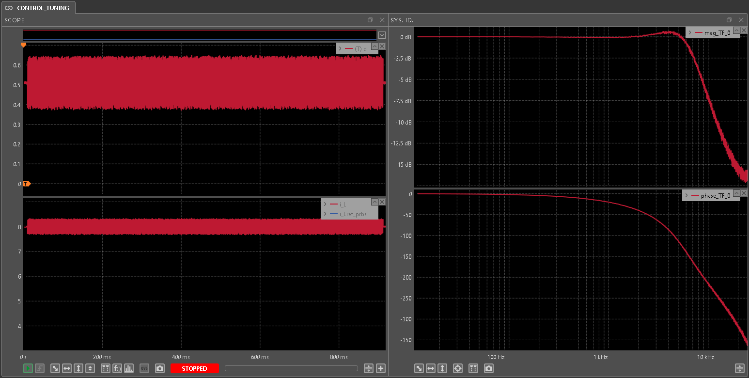
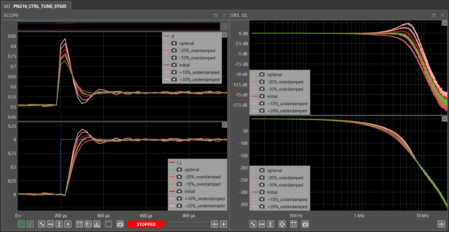
At this point, the overshoot is so small that the user might consider it acceptable and conclude the tuning procedure. Otherwise, it is possible to manually fine-tune the k_p and k_i gains to try improving the frequency response. For example, the user can slightly reduce the controller gains in case of an underdamped response, or slightly increase them otherwise. Cockpit’s snapshots feature simplifies comparing multiple acquisitions with different parameters. Moreover, the transient generator feature allows you to easily obtain the system step response. The following picture shows some tests conducted by increasing or decreasing the controller gains by the amounts indicated in the legend. Empirically, reducing the parameter gains by 7% yields a response close to a maximally flat one, with an acceptable step-response profile.

Conclusions

This note presented a frequency-domain PI controller tuning procedure. Starting from the frequency response measured in PN215, it showed how to derive all the necessary parameters from the Bode plot to apply the magnitude-optimum tuning criterion. The experimental validation yielded a slightly underdamped closed-loop frequency response, exposing the limitations of approximating this system as a first-order one. Finally, the procedure provided a simple way to manually adjust the controller gains and visually assess the response’s flatness, reducing the gap from the expected maximally flat response.