Table of Contents
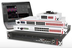
This user guide explains how to use imperix Cockpit to interact with imperix power converter controllers, namely the B-Box 4, B-Box RCP, B-Board PRO, the B-Box Micro, and the Programmable Inverter. The article gives an overview of the tools and features provided by Cockpit and how to use them.
For new users, it is recommended to read the article on Programming imperix controllers to get started with the imperix software development kit (SDK).
What is Cockpit
Cockpit is the monitoring software included with both the ACG SDK and CPP SDK. It is designed to facilitate the experimental testing of power electronics systems by leveraging the hardware capabilities of imperix programmable controllers.
The software provides various tools for interacting with imperix controllers and the user code running on them.
Connecting a user code with a controller
Uploading and running a custom code on an imperix controller starts with setting up a Cockpit project. Cockpit operates on a one user code – one project principle. Every project can only be connected to one device (or set of devices in case of a master-slave setup) at a time.
Cockpit, however, offers the flexibility of changing the user code that will be launched from a project, as well as the flexibility of reconnecting the project to a different device.
How to create a new project
To connect a user code with an imperix controller, creating a new project is required.
After the steps described in How to program the controller are achieved, Cockpit is automatically launched and a new project is created with a pre-filled project name and path to the user code.
Alternatively, it is also possible to manually open Cockpit and create a new project by clicking on the + button at the bottom of the left bar in the Projects perspective.
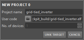
To finalize the project creation, the project must be linked to a Target. Clicking on the LINK TARGET button in the new project pane will automatically switch Cockpit to the Targets perspective.
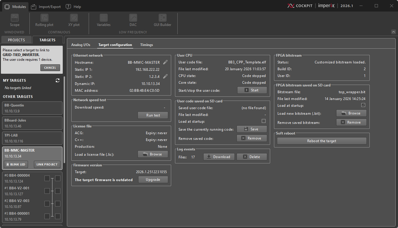
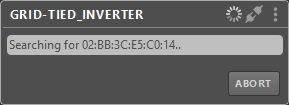
In the Targets perspective the left bar shows a list of imperix controllers detected by the host PC through Ethernet. Please refer to the chapter on How to connect the controller to the host PC to ensure your target is properly connected to the host computer.
The controllers are grouped based on their RealSync connections. The RealSync networks are then separated into MY TARGETS and OTHER TARGETS based on whether at least one device in the network is already linked to a Cockpit project.
Clicking on a controller will bring up the related Target view and show the button that allows linking the project to it. If the selected target is already linked, relinking will unlink the previous project and link the current one.
Once the project is linked, Cockpit will automatically shift back to the Projects perspective, where the newly created project pane will then appear in the left bar and a blank project view will be created.
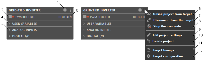
How use the project pane
The project pane offers a centralized view from which the user can pilot their imperix controller. It also allows quick access and an overview of all of the control variables defined in the user code.
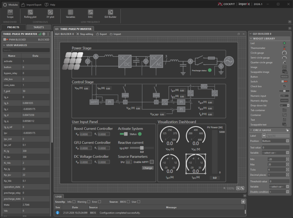
Upon linking, the project pane will automatically connect to the specified target, load, and start the user code (.elf file). The following image shows the project pane once it is connected to the target.
Interacting with the user code
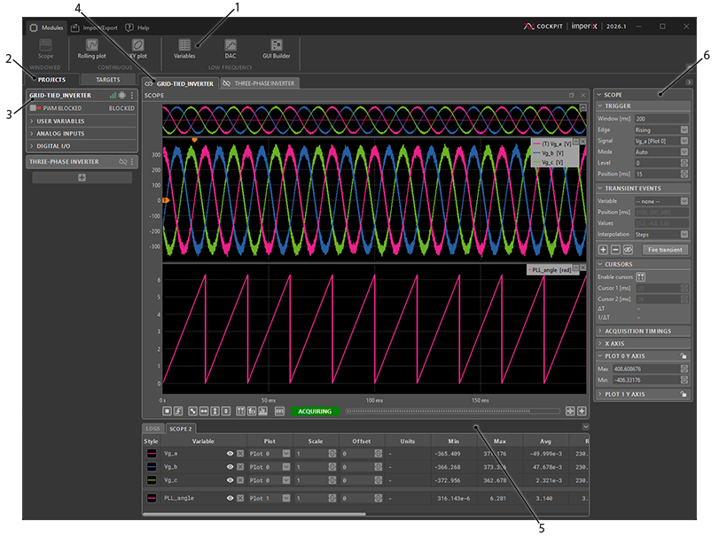
Once a project is created, the user has access to various control and monitoring modules that can be dragged and dropped from the top bar to the project view. The user can then freely rearrange and resize these modules inside the project view.
Scope module
This module allows the user to display control signals on an oscilloscope-like interface by capturing and plotting every sample of the scoped user variables. The acquisition is done at the control task rate (i.e. the main interrupt frequency of the controller), ensuring that each and every sample is scoped.
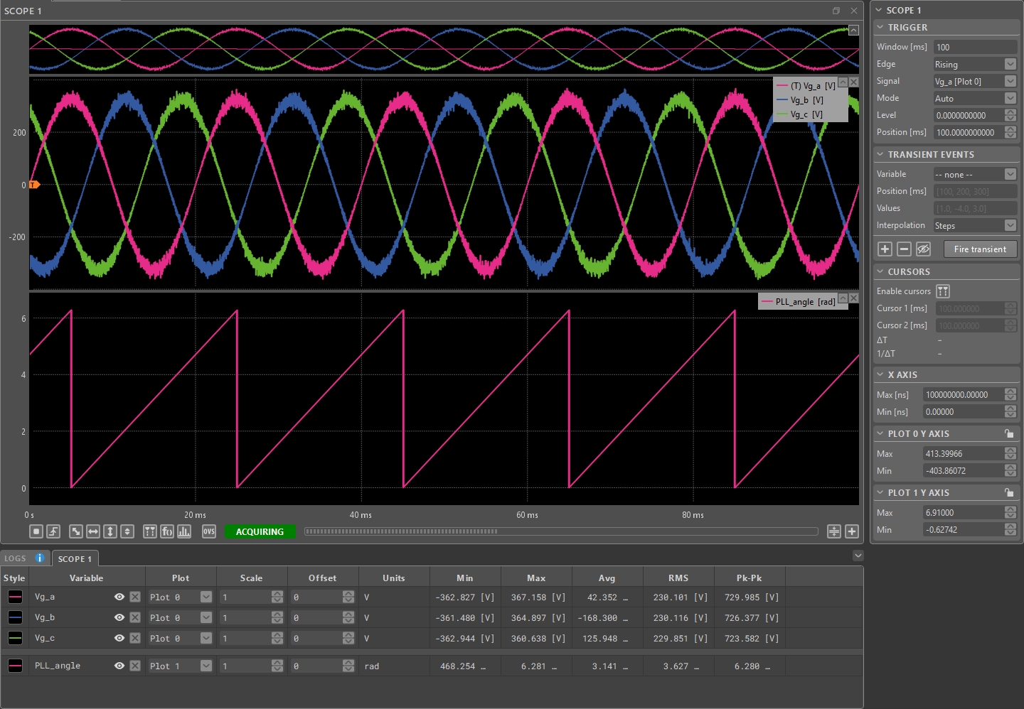
The Scope module offers many of the typical advanced oscilloscope features including Trigger configuration, Cursor measurements and Math functions. It also allows the user to preprogram and execute a sequence of value changes on Tunable variables while running their user code, through the Transient Generator mechanism.
A more detailed feature overview is available on the Scope module page.
Spectral Analyzer
The Spectral Analyzer allows the user to examine Scope variables in the frequency domain. This includes all of the user and math variables that are currently present in the module.
To add a variable to the Spectral Analyzer, add it to the Scope module and it will show up automatically. Conversely, removing a variable from the Scope will make it unavailable in the Spectral Analyzer as well.
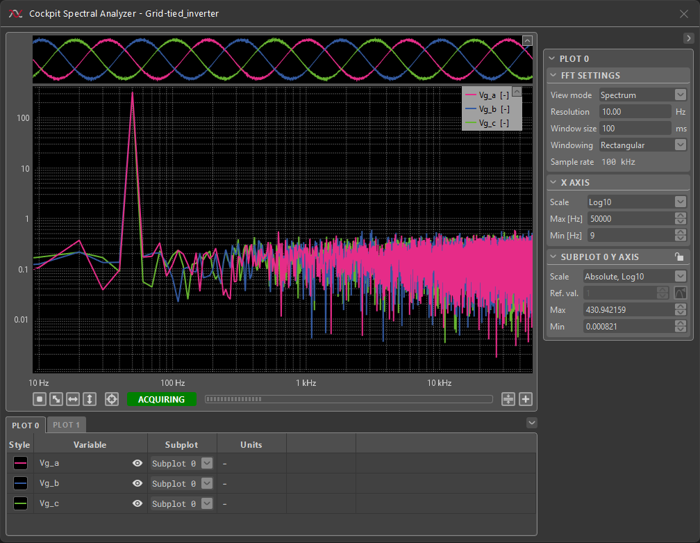
The Spectral Analyzer applies the Discrete Fourier Transform (DFT) on scoped data. The result can be examined in two forms – the Spectrum and Harmonics modes. The Spectrum mode offers an overview of the spectral content of all of the acquired data. In the Harmonics mode, the DFT is defined with respect to the fundamental harmonic frequency and the result is displayed in a way that makes it easier to compare the harmonic contents of acquired signals. This mode is accompanied by automated Total Harmonic Distortion (THD) measurements.
More details on the settings options and the underlying math are given on the Cockpit Spectral Analyzer page.
Rolling plot module
The rolling plot module allows for more long-term monitoring of the selected variables. A typical use case is monitoring the long-term evolution of the converter state in order to keep an eye on critical variables.
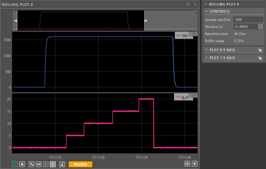
The sampling frequency of the Rolling plot can range from 10Hz up to the CPU control task frequency. The maximal amount of the recorded data depends on this value and the number of acquired variables. Once the allocated memory buffer fills up, the oldest acquired points will be deleted.
A closer look at the capabilities of the Rolling Plot module is provided on the Rolling Plot Module page.
XY plot module
The XY plot module allows for visualizing the relationship between two variables by plotting one against the other in a two-dimensional plane.
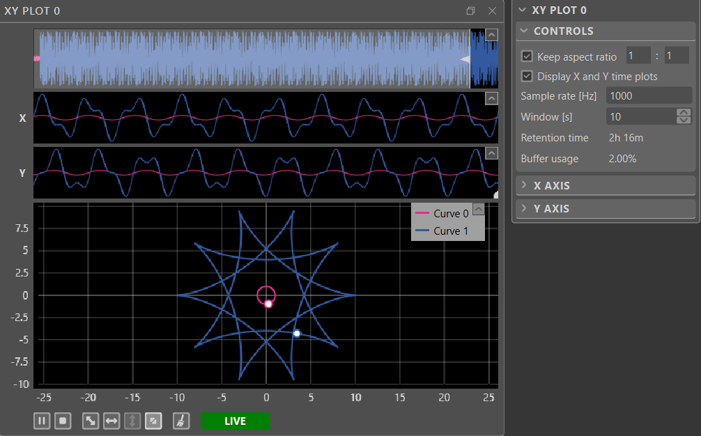
The sampling frequency of the XY plot can range from 10 Hz up to the CPU control task frequency. The maximal amount of the recorded data depends on this value and the number of acquired variables. Once the allocated memory buffer fills up, the oldest acquired points will be deleted.
The module also displays the X and Y variables over time in separate plots above the main XY plot, allowing for simultaneous monitoring of the temporal evolution of the signals.
A closer look at the capabilities of the XY plot module is provided on the XY Plot Module page.
Exporting plots from Cockpit modules
Cockpit offers the possibility to export the plotted signals acquired with the Scope and Rolling plot modules as a CSV or MAT file, or directly as a MATLAB figure.
For the scope module, Cockpit will export each and every sample of the scoped signals. As a reminder, the signal acquisition is performed at the control task rate. For the rolling plot module, Cockpit will also export each and every sample of the acquired signals, but at the sample rate selected in the rolling plot controls menu in the right bar.
To export data from a rolling plot or a scope module, click on the Export CSV, Export MAT, or MATLAB figure button located in the Import/Export tab of Cockpit’s top bar, as displayed below.
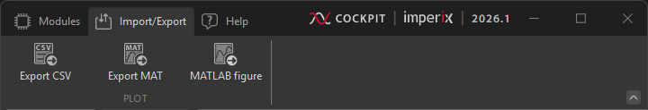
Data can also be exported through the context menus of the scope and rolling plot modules and the spectral analyzer window, accessible by right-clicking on the empty space in the plots.
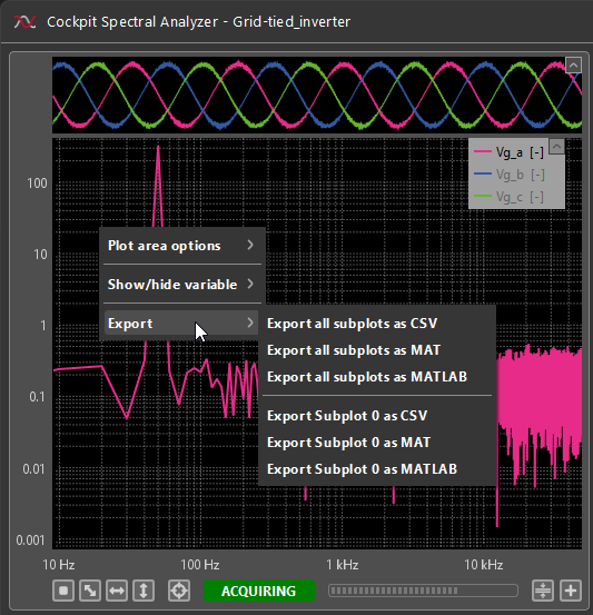
From the menu that appears, select the desired plots to export and choose the save location MATLAB figure or the CSV/MAT file. A MAT file is also saved when exporting data as a MATLAB figure.
Exporting as MAT file
Exporting as MAT file or MATLAB figure is done through the MAT 7.3 file format. This format is based on the HDF5 standard for hierarchical storing of data, allowing for partial saving and loading and better compression. This makes the export process more efficient in terms of time and memory in most cases, compared to CSV files.
A MAT file can be easily loaded to a MATLAB workspace by finding the file through the “Current folder” menu in MATLAB and double-clicking on it. The Working with MAT files exported from Cockpit article provides more information about the structure of the exported MAT files and different ways to load and save them.
Exporting as MATLAB figure
Exporting as MATLAB figure will first create and save a MAT file, as described in the previous section. Once the data has been exported as a MAT file, MATLAB is automatically launched with a new workspace set to the chosen folder. Finally, the MATLAB figure is automatically displayed.
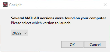
If several instances of MATLAB are installed on the computer, the user will be prompted to select the desired MATLAB version with the following pop-up message.
Variables module
The Variables module gives quick access to selected variables. It also allows modifying the user variables without rebuilding the control code. Additionally, it displays extra information on user variables, such as their minimum and maximum values.
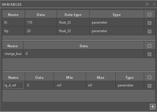
This module can contain one or more sections to sort the user variables conveniently.
- To add a new section, click the + button on the bottom left of the module.
- The columns displayed in a section can be managed by right-clicking on the section’s header and checking the desired columns.
- To add a variable to a section, drag and drop a variable from the project pane directly into the desired section.
- To remove a variable from a section, right-click on the variable and select “remove variable”.
- Signals connected to a Probe block are listed under the probe type, and signals connected to a Tunable parameter block are listed as parameter. Variables of type parameter can be modified in run-time by double-clicking on their value (Data column).
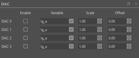
DAC module
The DAC module allows the user to apply a given variable to one of the four analog outputs of the B-Box RCP. The values applied to the analog output are specified in volts. The output range is -5V to 5V, and the output is saturated beyond these limits. Further hardware specifications are available in the B-Box RCP datasheet.
GUI Builder module
The GUI Builder module enables users to create custom dashboards for interacting with their user code running on an imperix controller.
The GUI Builder module page provides a more in-depth guide on building and using GUI Builder dashboards.
Interacting with the controller directly
While the modules are useful for interacting with the user code running on an imperix controller, Cockpit offers a range of other tools for monitoring and configuring the controller itself.
Information about a controller’s status and settings is centralized in the target view, which can be found by navigating to the corresponding device through the left bar in the Targets perspective. The target view displays controller information, sorted into three parts: the Analog I/Os, Target configuration and Timings tabs.
Configuring imperix controllers from Cockpit
Various controller info and configuration options can be found in Analog I/Os and the Target configuration tabs of the target view.
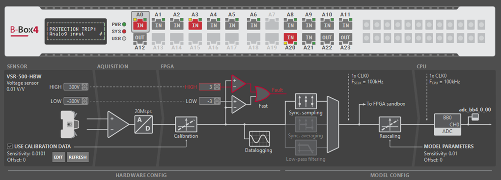
In the Analog I/Os tab, depending on the target imperix controller type, Cockpit offers different tools to set up the analog front-ends of the B-Box 4, B-Box RCP and B-Box Micro. Device-specific explanations are given below:
- Analog I/O configuration on B-Box 4
- Analog front-end configuration on B-Box RCP
- Analog inputs configuration on B-Box Micro
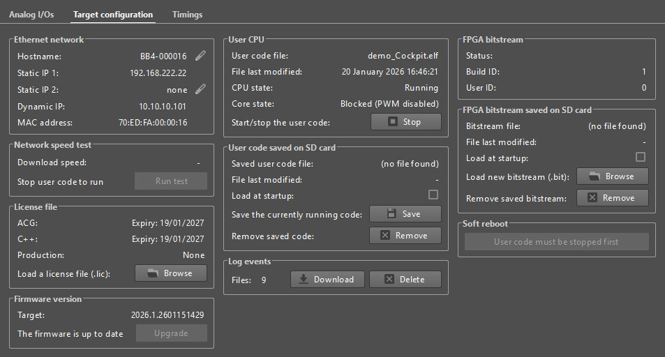
The Target configuration tab, also accessible from the three dots menu of a project pane, displays basic information about the controller and allows the user to manage licenses and firmware versions and interact with the controller memory by saving user codes, FPGA bitstreams and downloading controller logs from its SD card.
How to launch a user code at controller start-up
In some cases, it can be useful to automatically start a user code when turning on an imperix controller. To do so:
- Launch the user code and connect to the target as usual.
- Once the code is running on the target, open the Target configuration window from the three dots menu of the project pane.
- In the section User code saved on SD card, click on the Save the currently running code button to save the current code on the SD card inside of the controller.
- Click on the checkbox Load at startup to automatically launch the code when the controller is powered on.
This will save the control algorithm on the SD card inside the controller and automatically load and start it from the SD card at start-up.
How to load a custom FPGA bitstream
In some cases, it is interesting to offload all or parts of the computations from the CPU to the FPGA. Doing so often results in much faster closed-loop control systems. To do so:
- Launch the user code and connect to the target as usual.
- Once the code is running on the target, open the Target configuration window from the three dots menu of the project pane.
- In the section FPGA bitstream saved on SD card, click on the Browse button and select the desired bitstream. The bitstream will be uploaded into the SD card of the controller. A check in the Load at startup checkbox indicates that the target will load the imported customized bitstream at the next power cycle of the target instead of the standard one.
Further information on how to develop power converter control algorithms in FPGA can be found on the Getting started with FPGA control development page.
Monitoring the status of imperix controllers
Imperix controllers continually communicate with Cockpit to update the user about their status. Two main examples of this are the Timings tab in the target view and the Logs tab in the bottom bar.
Target timings
The Timings tab, also accessible from the three dots menu of a project pane, provides a graphical representation of the various computation and communication delays involved in the controller during run-time. It is particularly useful to observe the delays involved in the control dynamics of the system as explained in Identifying the discrete control delay (PN142). The control parameters, such as the \(K_p\) and \(K_i\) of a PI controller, can then be adjusted accordingly, as shown in Basic PI control implementation (TN105).
Below are screenshots of the Timings tab when running the model Central PV inverter (AN006) in two scenarios.
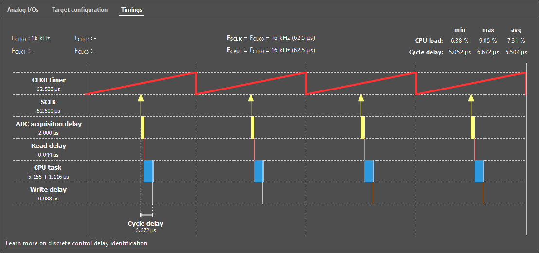

The timing graph accurately represents the delays involved in the execution of the user control code.
- CLK0 timer represents the clock generator counter. CLK0 is used as the time base for the sampling events and the control task routine execution. In most cases, the PWM modulators are also based on CLK0.
- SCLK shows the sampling events, i.e. the instants where the ADCs sample the input analog signals. In the example above, the sampling phase is set to 0.5, so the sampling occurs in the middle of the period of the PWM signals that are based on CLK0.
- ADC acquisition delay shows the delay between a sampling event and the availability of the values in the FPGA. It comprises the ADC acquisition delay and the transfer time of the read value to the FPGA. This value is 2000 ns in the B-Box RCP and 500 ns in the B-Box Micro and B-Board PRO. The appropriate value must be set from the CONFIG block.
- The Read delay shows the time needed to perform FPGA-to-CPU transfers. These tasks are executed right after the ADC results are available in the FPGA. The values transferred are typically the ADC measurements, the GPI values, or the angle decoder output.
- The CPU task shows the time the CPU spends executing the interrupt routine. To execute the CPU-to-FPGA transfers as early as possible (and reduce the overall response delay), the interrupt routine is separated into two phases:
- The control task execution is the time necessary to execute the user code and update the modulation parameters and other FPGA values. The CPU-to-FPGA transfers are executed right after, in parallel with the post-processing execution.
- The post-processing execution is the time necessary to perform all the tasks that are not directly involved in the control algorithm. It includes the datalogging execution, the CAN communication, etc.
- The Write delay shows the time needed to perform the CPU-to-FPGA transfers. These tasks are performed once the control task execution is over. The values transferred are typically the PWM modulation parameters (duty-cycle, phase), the GPO values, or the DAC values.
At the top of the tab, the following information is displayed:
- FCLK0, FCLK1, FCLK2, and FCLK3 show the configured frequency of the four Clock generators.
- FSCLK shows the FPGA sampling frequency and period. If the SCLK multiplier is configured, it will be displayed here. Check this article for more details .
- FCPU shows the routine execution frequency and period. If the control task Postscaler is applied, it will be displayed here. Note that the control task is always mapped on CLK0.
- The CPU load represents how much time the CPU spends in the interrupt routine relative to the period of CLK0. Safety mechanisms are implemented to detect CPU overload. An overload can result from a control algorithm being too complex or an execution frequency being too high. The min, max, and avg values are computed on a window of one second.
- The Cycle delay represents the delay between the sampling event and when the newly computed data are available in FPGA (ADC acquisition delay + FPGA-to-CPU transfers + control task execution + CPU-to-FPGA transfers). This value can be used to compute the control delay and the total loop delay, as explained in Identifying the discrete control delay (PN142). The cycle delay value is precisely measured directly from within the FPGA. The min, max, and avg values are computed on a window of one second.
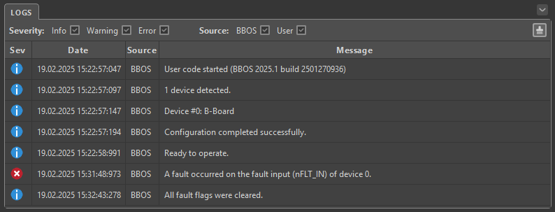
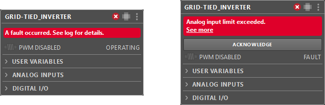
Logs tab
Messages from the controller to the user are displayed in the Logs tab in the bottom bar in the Projects perspective of Cockpit, and thus require the project to be connected to its controller.
The Logs tab displays every message reported by the controllers, including useful information such as misconfiguration details, software and hardware faults, or custom user messages.