Table of Contents
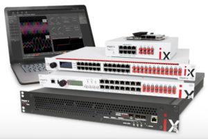
This user guide explains how to use Cockpit to interact with imperix controllers. The article provides an overview of the tools and features available in Cockpit, along with guidance on using them.
For users seeking getting-started assistance with the ACG SDK or the CPP SDK, a separate article is available in PN138, which focuses on programming imperix controllers. Specific quick-start guides are also available for each controller, such as the B-Box 4, B-Box 3, B-Box micro, or the TPI8032.
What is Cockpit
Cockpit is imperix’s real-time monitoring software. It is included in both the ACG SDK and CPP SDK. The software is designed to facilitate the experimental testing of power electronic systems.
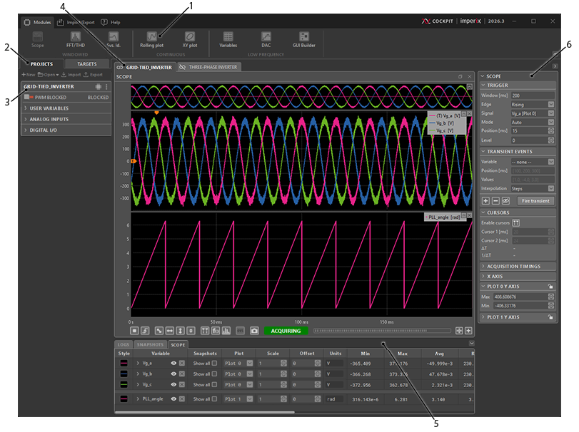
Cockpit’s interface is organized with six different sections:
Flashing a user code on a controller
Uploading and running a custom user code on a controller starts with setting up a Cockpit project. Projects are used to group a user code with its associated Cockpit configuration (monitored variables, arrangement of modules, etc.).
How to create a new project
Once a user code has been developed and compiled, Cockpit opens up automatically and invites the user to create a new project associated with the freshly compiled code. Instructions for the prior steps are provided in PN134 for Simulink/PLECS or PN148 for the C/C++ IDE.
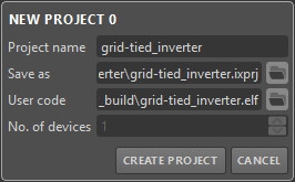
Alternatively, Cockpit can also be opened manually, and a new project can be created by clicking the + button at the top left of the left bar in the Projects perspective.
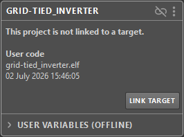
The project then needs to be linked to a target. Clicking the LINK TARGET button in the project pane automatically switches Cockpit to the Targets perspective, allowing this target to be selected from the available list. In multi-device configurations, the controllers are grouped based on their master-slave arrangement. If needed, please refer to PN138 to ensure the target is properly detected by the host computer.
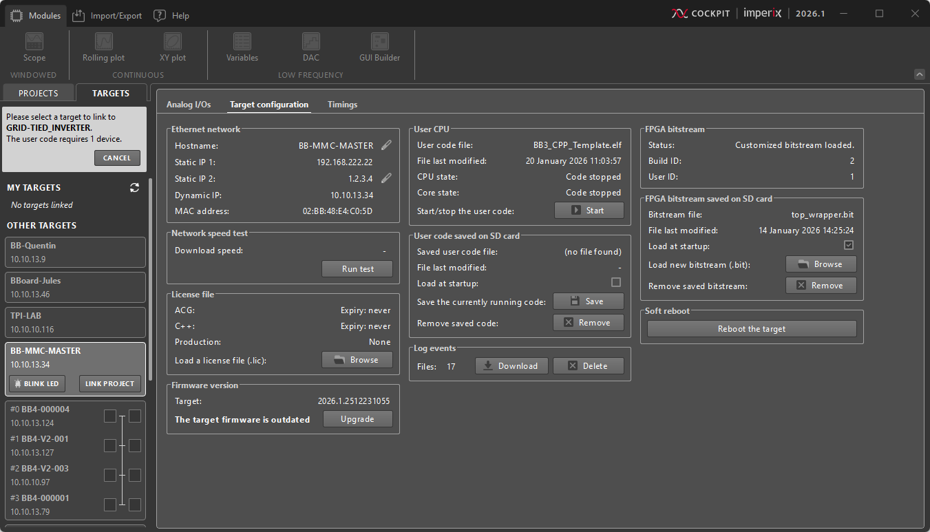
Clicking on a controller opens the corresponding target view and displays the button to link the project to it. If the selected target is already linked, relinking will unlink the previous project and link the current one. Once the project is linked, Cockpit automatically returns to the Projects perspective, where the newly created project pane appears in the left bar, and a blank project view is created.
How to manage projects
Each project can be linked to only one device (or a set of devices in a master-slave setup) at a time. However, Cockpit offers the flexibility to manipulate multiple projects simultaneously and re-link projects at will. If needed, the user code associated with a given project can also be changed.
When testing different algorithms or working with numerous targets, the Projects perspective can become crowded. To help keep the workspace organized or to ensure work is backed up, Cockpit provides options to open, close, import, or export projects.
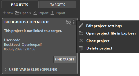
Every project is saved as a project file (.ixproj), which stores the workspace layout, the path to the user code, and the link to the target. These files can be managed using the following features:
- Opening and closing: Unused projects can be closed to hide them from the interface. The configuration data is safely stored in the .ixproj file, allowing it to be easily reopened whenever needed.
- Exporting and importing: To back up work or share it, entire workspaces can be bundled into a single .zip package. This includes the .ixproj file alongside all model files and assets, such as Simulink/PLECS models, MATLAB scripts, and snapshot data.
Detailed instructions are provided on the Working with Cockpit projects page.
How to use the project pane
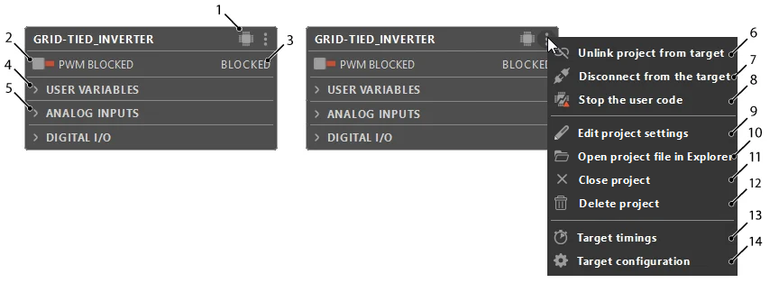
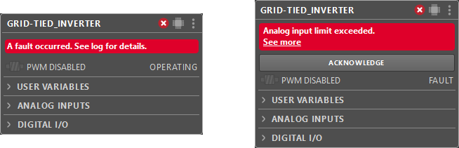
The project pane offers a centralized view from which the user can pilot their target during runtime. Additional tabs are also available, providing access to variables and oversampled I/O data.
Visualizing real-time data
Once a project is created, Cockpit modules can be dragged from the top bar into the project view and rearranged as needed. Cockpit features three different types of modules:
- Windowed modules capture data using a configurable trigger, similarly to an oscilloscope. When working with the transient generator, the capture can also be triggered manually. These modules capture data at the CPU control rate, and guarantee that no data point is ever missed. At the hardware level, the corresponding data is stored in a circular DDR buffer on the target and downloaded to the PC once the capture is complete.
- Continuous acquisition modules stream data from the target to Cockpit in real time. They capture data at a rate configurable from 10Hz to the CPU control rate, enabling long-term monitoring. These modules, however, depend on the quality of the Ethernet connection. If some data is missed, gaps may be present in the (timestamped) logs.
- Low-frequency modules operate by reading variables made available by the target via an internal OPC UA server, with a limited refresh rate (typically 10Hz). The GUI builder is the main module among them.
Windowed modules
These modules include the:
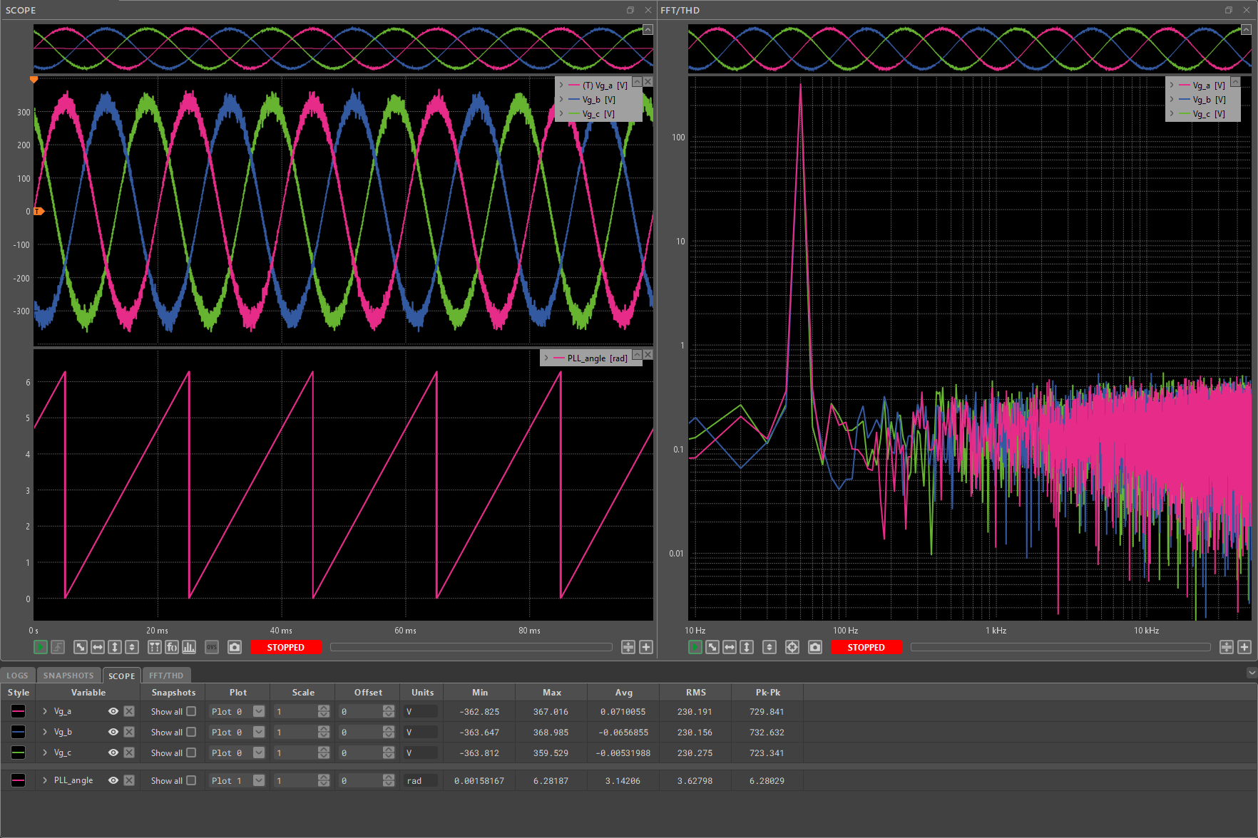
- Scope module, which displays variables on an oscilloscope-like interface offering trigger configuration, cursors with measurements, and custom math functions. It also supports a transient generator that can produce various reference steps and ramps. More details are available on the Scope module page.
- FFT/THD module, which lets the user examine scoped variables in the frequency domain. The Spectrum mode provides an overview of the spectral content of the whole window. In the Harmonics mode, the Fourier Transform is defined with respect to the fundamental harmonic frequency, displayed as a histogram, and paired with Total Harmonic Distortion (THD) measurements. More details are given on the FFT/THD module page.
Snapshots
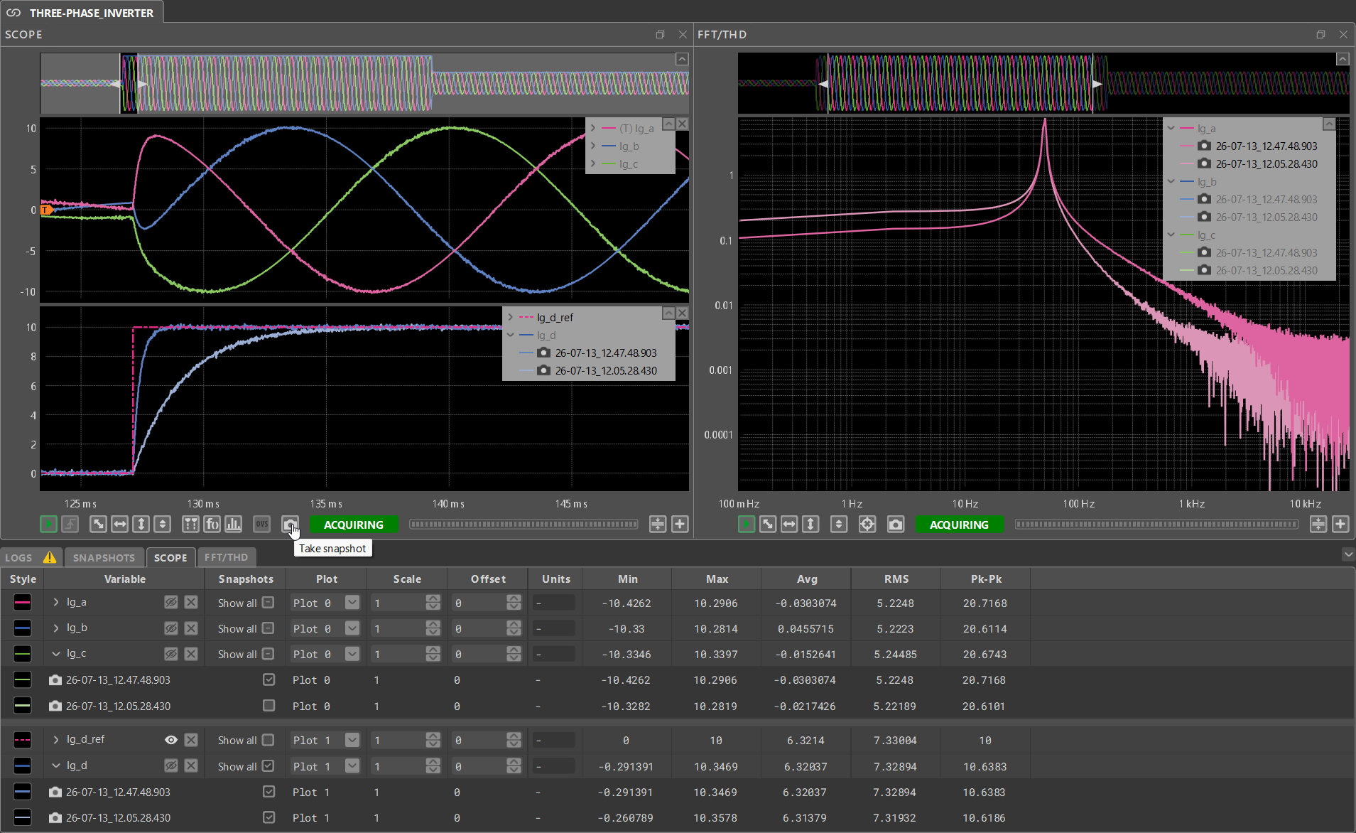
Acquired data can be saved for future comparison using Snapshots. To this end, clicking the snapshot button (camera icon) temporarily pauses data acquisition and saves the data currently displayed. Data from previous snapshots appear in collapsible menus next to each variable and can be displayed by clicking the corresponding eye icon.
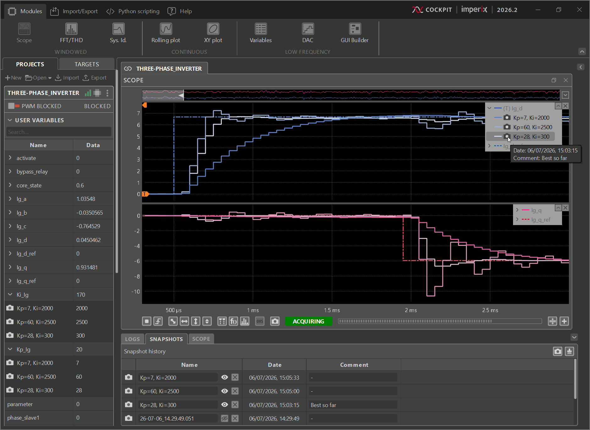
Snapshots are listed and can be manipulated from the dedicated tab in the bottom pane. They can notably be renamed, providing a simple way to keep track of the conditions associated with their capture. Snapshots can also be deleted.
Snapshots are recorded as MAT files (.mat) and saved in a folder next to the project file (.ixproj). They are automatically exported along with other project files. More details on the snapshot’s structure and attributes are provided in PN141.
Continuous acquisition modules
These modules include the:
- Rolling Plot module, which allows monitoring the long-term evolution of variables. A closer look at the module’s capabilities is available on the Rolling Plot Module page.
- XY Plot module, which lets the user monitor the long-term evolution of 2 variables against each other.
A closer look at the capabilities of the XY Plot module is provided on the XY Plot Module page.
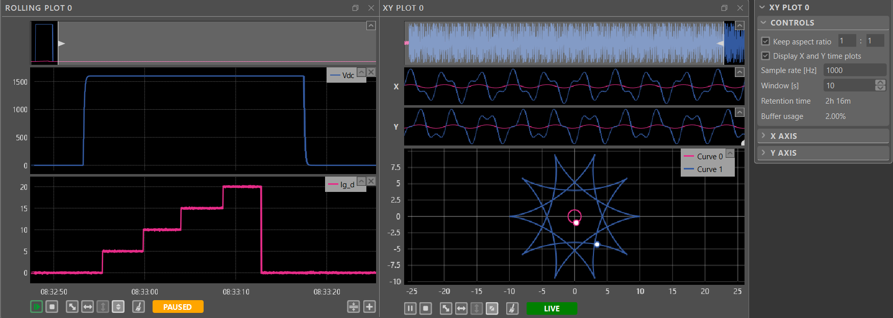
Multiple instances of these modules can be added to the same project, each with its own acquisition rate. Each instance has its own allocated memory buffer which, once full, starts erasing the oldest data. The maximum recording length depends on the selected acquisition rate and the number of variables acquired.
Exporting plots from Cockpit modules
Cockpit offers the possibility to export the plotted signals as a CSV file, MAT file, or directly as a MATLAB figure. The data from all plotting modules are saved as-is, with each acquired sample recorded.
To export data from a plotting module, click on the Export CSV, Export MAT, or MATLAB figure button located in the Import/Export tab of Cockpit’s top bar, as displayed below. Data can also be exported from the plotting module’s context menus, accessed by right-clicking the empty space in the plots.
From the menu that appears, select the desired plots to export and choose the save location: a MATLAB figure or a CSV/MAT file. A MAT file is also saved when exporting data as a MATLAB figure. When large amounts of data are at stake, exporting to a MAT file is recommended.

When exporting as a MATLAB figure, a MAT file is first created and saved. Then, MATLAB is automatically launched with its path set to the destination folder. Finally, the MATLAB figure is automatically displayed.
Low-frequency modules
GUI Builder module
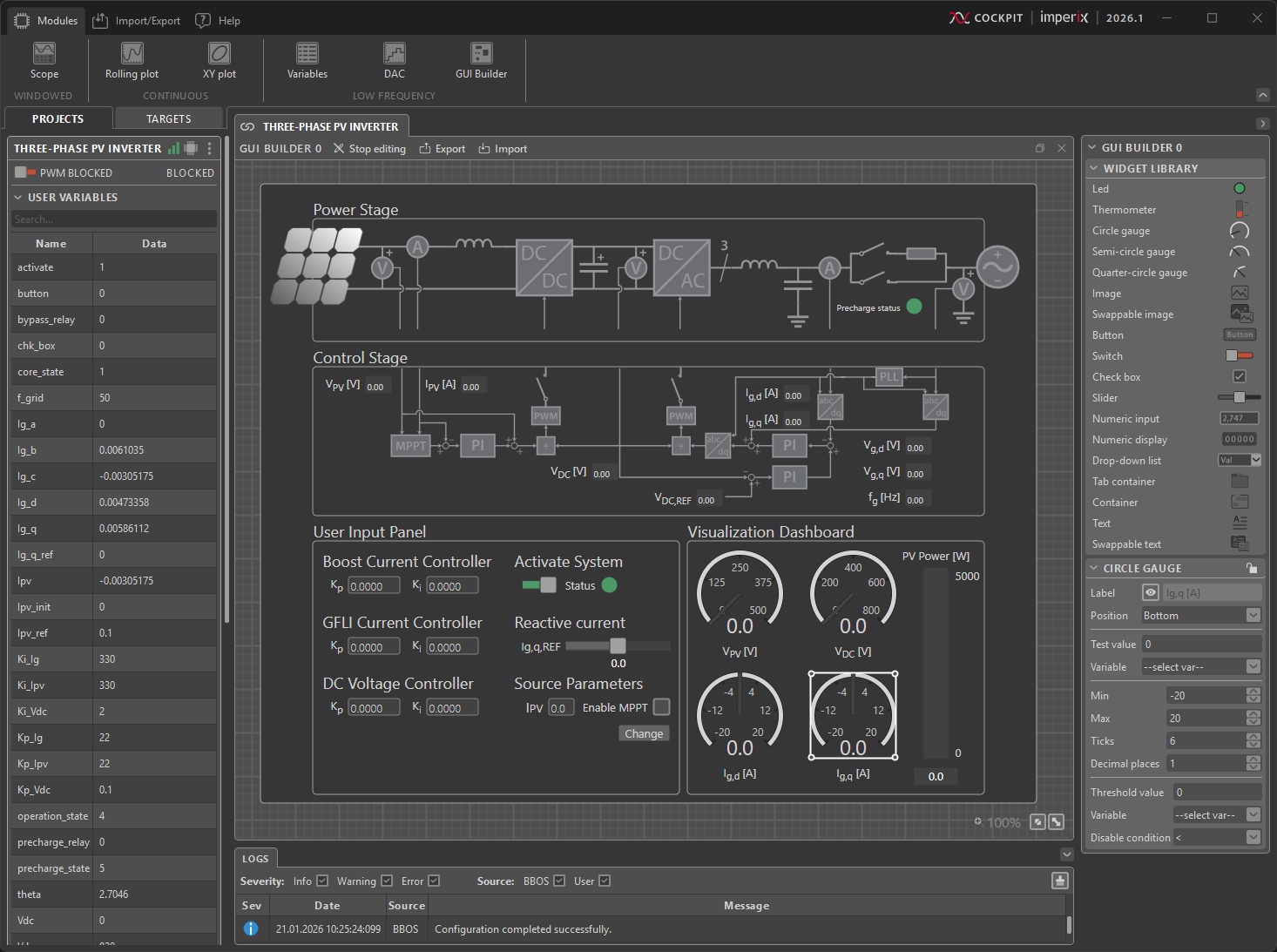
The GUI Builder module enables users to create custom dashboards to interact with the user code at runtime. Dashboards can also be built in advance when no target connection or active code is present. The GUI Builder module page provides a more in-depth guide on building and using dashboards.
Variables module
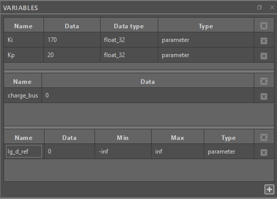
The Variables module provides quick access to selected variables along with basic statistics. This module can be arranged with distinct sections to conveniently sort variables. To add a new section, click the + button on the bottom right of the module. The columns displayed in a section can be managed by right-clicking the section header and selecting the desired columns.
DAC module
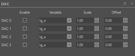
The digital-to-analog (DAC) output module is a legacy module specific to the B-Box 3. It allows a given variable to be applied to one of the device’s four analog outputs, with the value specified in volts. The output range is -5V to 5V. Further hardware specifications are available in the corresponding datasheet. If a DAC block is used in the user code and the DAC module is also used in Cockpit, Cockpit takes precedence.
With the B-Box 4, analog outputs can only be configured using DAC blocks.
Interacting with the controller
Information about controller status and settings is centralized in the target view, which is accessible by switching to the Targets perspective (left pane). This view is organized into three tabs:
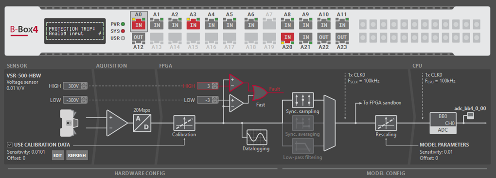
- The Analog I/Os tab provides a remote view of the device’s front panel, showing the current configuration and indicating the origin of the fault, if any.
- The Target configuration tab provides information on the IP configuration, the validity of the software license, and the firmware version. This is also where custom FPGA bitstreams can be loaded and event logs retrieved.
- The Timings tab shows detailed information on the device’s acquisition, processing, and data transfer timings. Knowing this information is often essential to properly identify the total closed-loop control delay.
Analog I/Os tab
In this tab, depending on the target imperix controller type, Cockpit provides different tools for configuring the analog front end. Device-specific explanations are given in separate documents:
| Controller | Configurable through | Device-specific documentation |
|---|---|---|
| B-Box 4 | – Device front-panel (LCD+button) – Cockpit Analog I/O tab | PN252 |
| B-Box 3 (RCP) | – Device front-panel (LCD+button) | PN105 |
| B-Board 3 (PRO) | N/A | N/A |
| B-Box 3 micro | – Cockpit Analog I/O tab | PN106 |
| TPI8032 | N/A | PN190 |
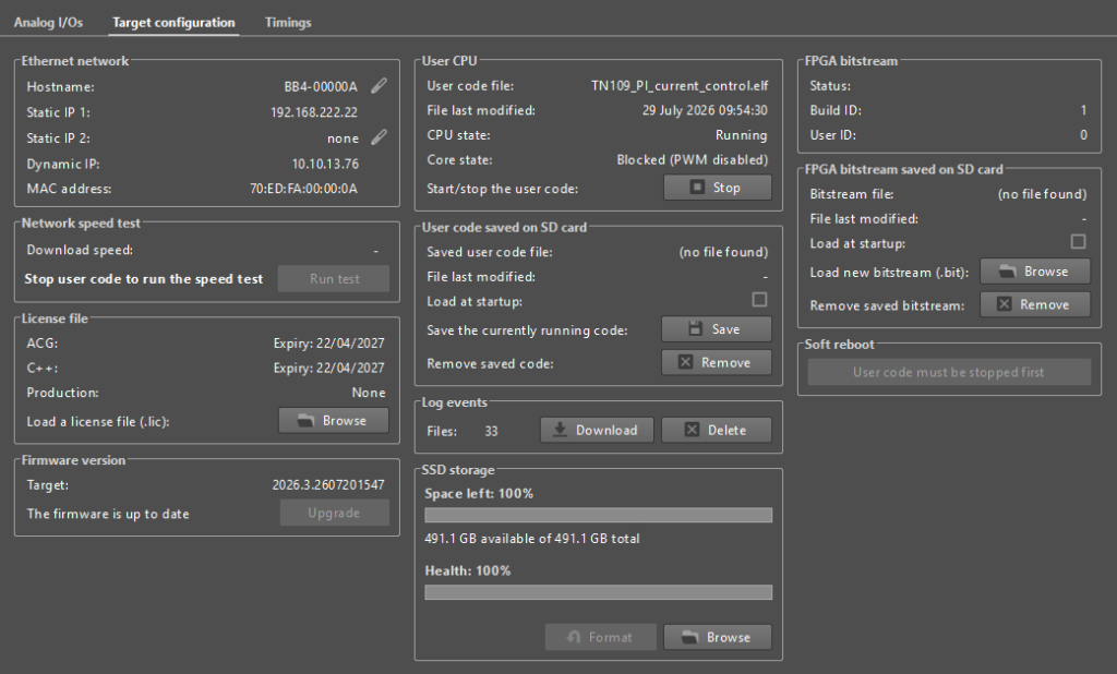
Target configuration tab
This tab regroups several firmware-related information and configuration options. This is also where the device’s storage units can be accessed to load a license file or bitstream, or load/save logs and data profiles.
How to change the device’s IP address
Imperix controllers have two static IPs and one dynamic IP, automatically assigned via DHCP.
In most situations, this doesn’t require the user’s attention, as the Ethernet configuration behaves well automatically. Nonetheless, if desired, the second IP can be modified at will by clicking the edit icon. (The first static IP serves as a safeguard/backup value and cannot be changed.)
How to load a software license
The use of the ACG SDK or the CPP SDK is subject to a (paid) license. The validity of this license is checked at the code startup, on the controller. This permits installing and using the software on an unrestricted number of computers. More information about imperix’s licensing policy is available in PN160.
A license file can be uploaded easily from the Target configuration tab by clicking the Browse button.
How to make the user code automatically launch at start-up
In some cases, it can be useful to automatically start user code when the controller is turned on. To do so:
- Launch the user code and connect to the target as usual.
- In the User code saved on SD card section, click the Save the currently running code button to save the current code to the SD card.
- Click the Load at startup checkbox to automatically launch the code when the controller is powered on.
How to load a custom FPGA bitstream
Information on developing custom logic in the user-programmable FPGA area can be found on the Getting started with FPGA control development page. To load the resulting bitstream onto the controller:
- Launch the user code and connect to the target as usual.
- Once the code is running on the target, open the Target configuration window from the three-dot menu in the project pane.
- In the section FPGA bitstream saved on SD card, click on the Browse button and select the desired bitstream. The bitstream will be uploaded to the controller’s SD card. Checking the Load at startup checkbox indicates that the target will load the imported customized bitstream at the next power cycle, instead of the standard one.
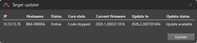
How to upgrade the firmware
Timings tab
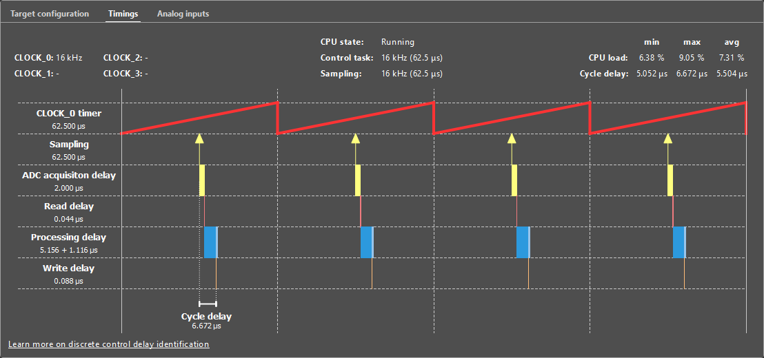
This tab provides a graphical representation of the various delays experienced by the controller at runtime. It is notably useful to identify the total control delay, as documented in PN142. The control parameters, such as the \(K_p\) and \(K_i\) of a PI controller, can then be adjusted accordingly, as further developed in TN105.
Below are screenshots of the Timings tab for the Central PV inverter (AN006) model executed at two different control rates.
 Central PV inverter running at 16 kHz
 Central PV inverter running at 160 kHz
The timing graph accurately represents the delays incurred during execution of the user control code.
- CLK0 timer represents the clock generator counter. CLK0 is used as the time base for sampling events and for executing the control task execution. In most cases, the PWM modulators are also based on CLK0.
- SCLK indicates the sampling events, namely the instants at which the ADCs sample the analog inputs. In the example above, the sampling phase is set to 0.5, so sampling occurs midway through the PWM period.
- ADC acquisition delay shows the delay between a sampling event and the availability of the values in the FPGA. It comprises the ADC acquisition delay and the time required to transfer the read value to the FPGA.
- The Read delay shows the time needed to perform FPGA-to-CPU transfers. These tasks are executed right after the ADC results are available in the FPGA.
- The CPU task shows the time the CPU spends executing the control algorithms. This is separated into two phases:
- The control task execution represents the time necessary to execute the user code and update the modulation parameters and other FPGA values. The CPU-to-FPGA transfers are executed immediately afterward, in parallel with the post-processing.
- The post-processing execution represents the time required to perform all tasks not directly involved in the control algorithm.
- The Write delay indicates the time required to perform CPU-to-FPGA transfers. These tasks are performed once the control task has finished executing. The values transferred are typically the PWM modulation parameters (duty-cycle, phase), the GPO values, or the DAC values.
More information about how imperix controllers process data is given in PN261. Basic sampling configurations are also further described in PN259.
At the top of the tab, the following information is displayed:
- FCLK0, FCLK1, FCLK2, and FCLK3 show the configured frequency of the four clock generators.
- FSCLK shows the FPGA sampling frequency and period. If the SCLK multiplier is configured, it is displayed here. PN259 provides more details on common and advanced sampling configurations.
- FCPU shows the execution frequency and period of the routine. If the control task Postscaler is applied, it will be displayed here. Note that the control task is always mapped on CLK0.
- The CPU load represents how much time the CPU spends in the interrupt routine relative to the CLK0 period. Safety mechanisms are implemented to detect CPU overload.
- The Cycle delay represents the time between the sampling event and the availability of the newly computed data in the FPGA (ADC acquisition delay + FPGA-to-CPU transfers + control task execution + CPU-to-FPGA transfers). This value can be used to compute the control delay and the total loop delay, as explained in PN142. The cycle delay is measured directly within the FPGA. The min, max, and avg values are computed over a 1-second window.
Logs tab
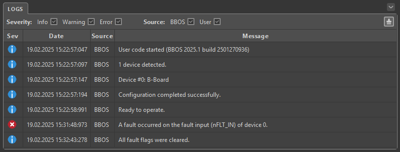
Log messages are displayed in the Logs tab in the bottom bar in the Projects perspective of Cockpit. The Logs tab displays every message reported by the controllers, including useful information such as misconfiguration details, software and hardware faults, or custom user messages.
 By Stéphane Lovejoy • January 19, 2024 • PN304
 By Julien Orsinger • April 6, 2022 • SD050