Table of Contents
This technical note provides an overview of Active Power Filters (APFs) designed for harmonic mitigation and specifically targeting three-phase grid-connected inverters.
The note begins by introducing various APF topologies and control schemes. Then, it presents a practical implementation and experimental validation of a shunt active power filter using the TPI8032. This example adresses the case of a nonlinear load connected to a three-phase grid.
Additionally, ready-to-use Simulink and PLECS files are available for download.
Software resources
The implementation of an shunt active power filter in Simulink and PLECS can be found below.
What is an Active Power Filter (APF)
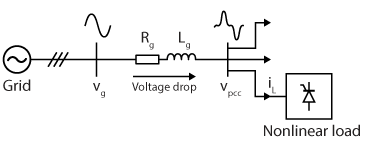
Ideally, an electrical grid should supply loads with a purely sinusoidal voltage. However, many nonlinear loads draw distorted currents. Such as variable-speed drives, computer power supplies and industrial converters. As these non-ideal currents flow through the line impedance, they create voltage drops at specific frequencies (harmonics), leading to voltage distortion at the load terminals. This phenomenon degrades power quality and increases energy losses. This is illustrated below.
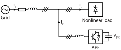
To mitigate these issues, active power filters provide a dynamic and effective solution by injecting compensating currents, which sum-up with the nonlinear load current as to create a sinusoidal current at the point of common coupling (PCC) [1]. This mitigate the total amount of harmonics distortion and enhancing the overall power quality of the grid. Moreover, unlike traditional passive filters, APFs can dynamically adapt to varying load conditions and act as a STATCOM, providing reactive power compensation when needed.
Finally, active power filters are also crucial for ensuring compliance with harmonic standards such as IEEE 519 or IEC 6100.
Topologies of Active Power Filters
Active Power Filters can be classified based on their hardware configurations and the objectives of their application [2]. The main topologies include the following ones :
1. Shunt Active Power Filter (SAPF)
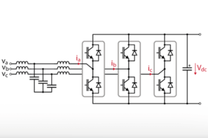
This is the most widely used topology, designed to eliminate current harmonics, compensate reactive power, and, in some cases, equilibrate unbalanced currents. In addition, this topology makes it easy to scale the output power. SAPF are installed in parallel with the load and injects compensating currents of equal magnitude but opposite phase to the harmonic currents generated by the load. This method is highly effective in damping harmonic propagation within power systems. The figure below illustrates a shunt active power filter connected to the grid.
2. Series Active Power Filter
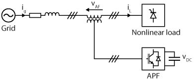
This topology connects in series with the power line through a transformer and primarily addresses voltage-related issues such as harmonics, negative-sequence voltage, and flicker. Series APF are generally placed close to electrical installations in order to attenuate voltage harmonics propagated by line resonances. The figure below shows a serie active power filter connected to a grid.
3. Hybrid Active Power Filter
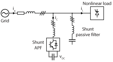
Hybrid APFs combine active and passive filtering elements to achieve cost-effective harmonic mitigation. For instance, a passive filter can handle lower-order harmonics, while the active component compensates for higher-order harmonics and dynamic conditions. This topology is widely used for high-power applications due to its reduced cost and improved efficiency. The figure below shows a hybrid active power filter connected to a grid.
4. Unified Power Quality Conditioner (UPQC)
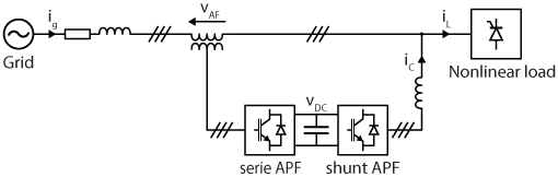
This advanced topology integrates both series and shunt APFs into a single system. The UPQC compensates for both voltage and current distortions simultaneously, offering comprehensive power quality solutions. While highly effective, UPQCs are more complex and costly, making them suitable for critical applications requiring superior power quality. The figure below shows an UPQC connected to a grid.
Control strategies of a shunt APF
The control strategy of Active Power Filters often consists of three key steps in order to achieve a proper harmonic mitigation. The figure below illustrates these processes, and the following sections describe them.
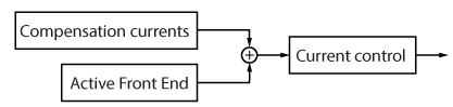
The first and most important step is the generation of compensation current signals. These signals correspond to the corrective currents that, when combined with the nonlinear load currents, produce a sinusoidal current on the grid side. Careful attention to the estimation of compensation signals is important, as this step directly influences the APF’s ability to reduce harmonic distortion.
The second step is the control of the DC bus voltage. This step acts as an Active Front End (AFE) and generates an additional current reference, which ensures that the DC bus voltage remains at the desired level. However, if the DC bus is powered by an external source, this regulation is unnecessary, as the voltage is already maintained independently. Together with the first step, the total current reference that the converter must follow are defined.
The third and final step is the application of the current control to ensure that the APF tracks the current references calculated in the previous steps. The selection and tuning of the controller require special attention, as APF current references have a distinct waveform that includes high-order harmonics (i.e., high-frequency components).
Estimation of the compensation signals
The estimation of compensation signals plays a key role in active power filter control, directly impacting performance and computational complexity. Different methods exist to estimate these signals, which can be broadly classified into two main approaches: time-domain methods and frequency-domain methods.
Frequency-domain methods use spectral analysis to identify and eliminate harmonics but require high computational resources, making them difficult to use for real-time applications. Consequently, these methods are out of the scope of this article.
Time-domain techniques extract compensation signals instantly from distorted waveforms, offering fast response and simple implementation but are limited to single-point corrections . In practice, these algorithms measure the current drawn by the nonlinear load, isolate harmonics using a high-pass filter, and inject the high-frequency components (>50 Hz) back into the grid with same amplitude but opposit phase. As a result, the APF supplies the non-sinusoidal and high-frequency currents drawn by the nonlinear load. This prevents the grid from bearing these distortions.
Among the various time-domain techniques, the most widely used is the instantaneous P-Q strategy [3], which is detailed in the section below.
Instantaneous P-Q theory for active power filters
The Instantaneous P-Q theory, also known as the P-Q strategy, aims to ensure that the active and reactive powers drawn from the grid do not oscillate. This implies that the currents drawn from the grid must be perfectly sinusoidal, assuming the voltage is also ideal. To achieve this, the P-Q strategy first calculates the instantaneous active and reactive powers consumed by the nonlinear load using Eq. (1).
$$ (1) \quad \begin{bmatrix} p_L\\ q_L \end{bmatrix} = \begin{bmatrix}
v_{g,\alpha}&v_{g,\beta}\\
-v_{g,\beta} & v_{g,\alpha}
\end{bmatrix} \begin{bmatrix}
i_{L,\alpha}\\
i_{L,\beta}
\end{bmatrix} $$
As a result, when the load currents are not purely sinusoidal at the fundamental frequency (i.e., they contain negative-sequence components or harmonics), the instantaneous active and reactive powers fluctuate instead of remaining constant. Consequently, the formulation expresses the active and reactive powers as the sum of a constant and an oscillating component, as follows :
$$ (2) \quad p_L = \tilde{p}_L + \bar{p}_L \quad \quad q_L = \tilde{q}_L + \bar{q}_L$$
To ensure that the grid supplies only a constant power, the role of the APF is to inject the oscillating power components consumed by the nonlinear load. This compensation corresponds to :
$$ (3) \quad p^*_{APF} = -\tilde{p} _{L} \quad \quad q^*_{APF} = -\tilde{q} _{L} $$
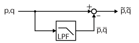
Therefore, it is necessary to determine the instantaneous values of \(\tilde{p} _{L}\) and \(\tilde{q} _{L}\). This is achieved using a high-pass filter (HPF), which removes the constant power components from the instantaneous power signals, leaving only the oscillating terms. The HPF can also be implemented using a low-pass filter (LPF), such as a Butterworth filter, as follows:
Using these oscillating components as references for the APF leads to the grid-side power shown in Eq. (4).
$$ (4) \quad p_{g} = \tilde{p} _{L} + \bar{p} _{L} + \underbrace{\tilde{p} _{APF} }_{\approx -\tilde{p} _{L} } + \bar{p} _{APF} \approx \bar{p} _{L} + \bar{p} _{APF}$$
From the equation above, we can conclude that the instantaneous power drawn from the grid remains constant, ensuring that the grid current is purely sinusoidal and free of distortion. Moreover, since the shunt APF operates by controlling currents rather than power, the compensating currents \(i^*_{c,abc}\) must be derived from the power references. This is achieved by inverting Eq. (1), resulting in the following expression :
$$ (5) \quad \begin{bmatrix} i^*_{c,\alpha}\\ i^*_{c,\beta} \end{bmatrix} = \begin{bmatrix}
v_{g,\alpha}&v_{g,\beta}\\
-v_{g,\beta} & v_{g,\alpha}
\end{bmatrix}^{-1}
\begin{bmatrix}
p^*_{APF}\\
q^*_{APF}
\end{bmatrix}$$
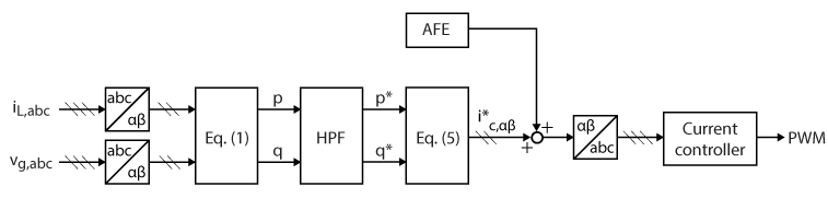
This equation allows the APF to compute the instantaneous reference currents required to inject the appropriate compensating currents. The illustration below shows the complete process of the P-Q strategy.
Active front End
Powering the DC bus of an Active Power Filter externally can be costly and impractical. Since the APF is connected to the grid, it can self-power by drawing energy from the grid while using its DC bus as a buffer. This is achieved through an Active Front End (AFE), which regulates the DC bus voltage. Since the APF reinjects all the absorbed active power back into the same grid, the AFE technically compensates only for the system losses. This control step generates a current reference that is simply added to the APF’s existing reference.
For details on tuning and implementation, refer to the Active Front End technical note.
Current control for an active power filter
In a three-phase grid, nonlinear loads typically generate odd non-triplen harmonics of the form 6n ± 1 (e.g., 5th, 7th, 11th, 13th,…). These high-frequency harmonics can only be effectively compensated if they fall within the bandwidth of the current controller. Therefore, a high-bandwidth controller, or one with high gain at these harmonic frequencies is crucial for optimal APF performance.
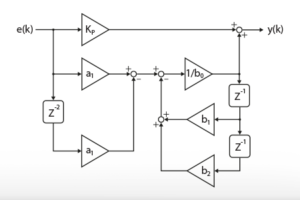
The literature presents various current controllers suitable for APFs, including PI, PI + Resonant, Predictive, Deadbeat, and Hysteresis controllers. Among these options, this technical note uses a Proportional-Resonant (PR) controller, specifically tuned for the four dominant harmonics (h = 5, 7, 11, 13).
For details on implementation and tuning, refer to the PR Controller technical note.
Implementation of a shunt APF with a TPI8032
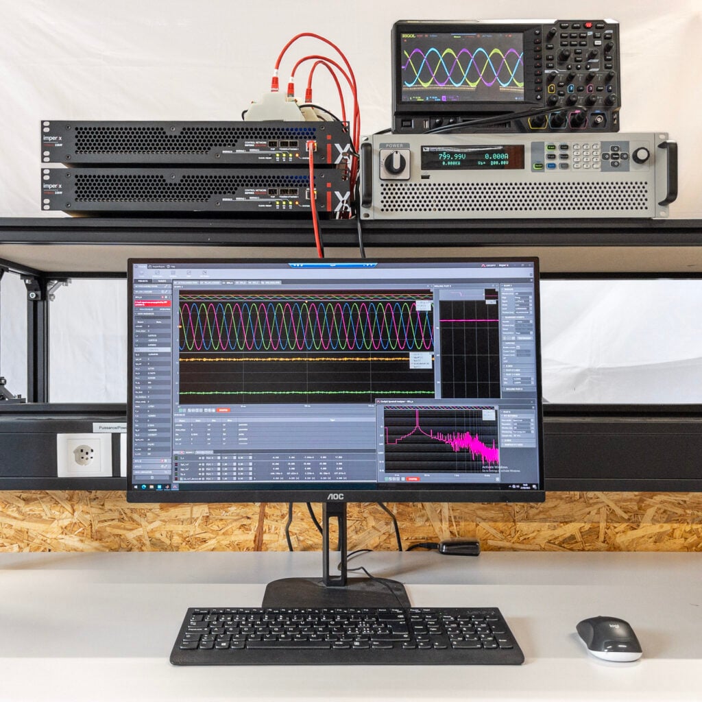
Experimental setup
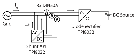
The experimental setup in this article consists of two TPI8032 and three DIN50A current sensors, all connected to the same grid. The first TPI8032 operates as the Active Power Filter (APF), while the second emulates a diode rectifier (nonlinear load). Additionally, the APF uses three current sensors to measure the currents drawn by the nonlinear load. Finally, the DC power supply absorbs the power from the emulated diode rectifier.
| Control and switching frequency | 50 kHz |
| DC bus voltage | 800 V |
| Grid voltage (L to N) | 230 VRMS |
It is also possible to configure the two TPI8032 in a master-master setup, allowing the APF to use the current measurements from the diode rectifier emulator, instead of requiring external current sensors. This reduces the need for additional hardware.
Experimental results
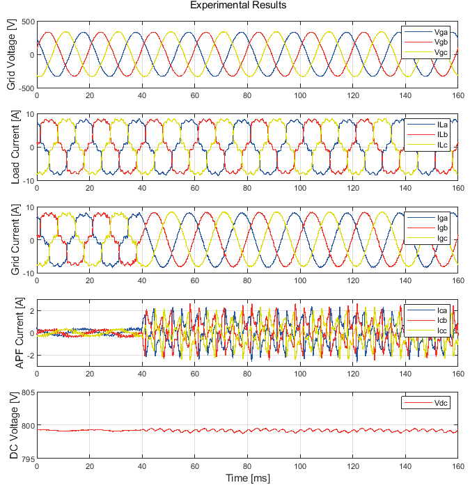
The figure below presents the experimental results, displaying the currents from the diode rectifier and the APF, the grid voltage and current, as well as the DC voltage of the APF.
First, the diode rectifier draws a distorted current while the APF is connected to the grid but inactive. At t = 40 ms, the APF activates its control, injecting compensating currents with a specific waveform. From this moment, the grid currents, obtained by summing the APF and diode rectifier currents, become sinusoidal. This demonstrate the effectiveness of the APF for harmonics mitigation.
Additionally, the figure below illustrates the harmonic content of the grid current before and after APF activation, highlighting the combined performance of the compensation current calculation (Instantaneous P-Q theory) and the current controller.
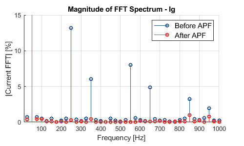
Finally, the 17th and 19th (red in figure, at 850Hz and 950Hz) harmonics appear less attenuated compared to the first four dominant harmonics. This is due to the fact that the PR controller was specifically tuned for the 5th, 7th, 11th, and 13th harmonics, while higher-order harmonics are only attenuated by the proportional gain of the PR controller.
Academic references
[1] H. Akagi, “Active Harmonic Filters,” in Proc. IEEE, Vol. 93, N°. 12, pp. 2128-2141, Dec. 2005.
[2] B. Singh, K. Al-Haddad and A. Chandra, “A review of active filters for power quality improvement,” in IEEE Transactions on Industrial Electronics, Vol. 46, N°. 5, pp. 960-971, Oct. 1999
[3] M. I. M. Montero, E. R. Cadaval and F. B. Gonzalez, “Comparison of Control Strategies for Shunt Active Power Filters in Three-Phase Four-Wire Systems,” in IEEE Trans. on Pow. Elec., Vol. 22, N°. 1, pp. 229-236, Jan. 2007.