Proportional resonant controller

This article presents the basic theory of operation of proportional resonant controllers, and introduces a possible implementation for the control of single-phase voltage source inverters. The corresponding software is given for Simulink and C++ code and is made available for download.

What is a proportional resonant controller?

Proportional resonant controllers (abbreviated PR controllers) are a particular type of transfer function that are often implemented for the closed-loop control of systems with a sinusoidal behavior. As their name indicates, they possess both a proportional and a resonant term, which can be tuned independently. When needed, additional resonant terms can also be added to attenuate specific harmonics. 

In power electronics, proportional resonant controllers (PR) have attracted significant interest for AC current/voltage control applications due to their performance and simple implementation.

Benefits of proportional resonant controllers

In DC applications, conventional

PI controllers provide excellent performance, notably a minimal steady-state error, thanks to the (almost) infinite DC gain provided by the integral control action. However, in AC applications, PI controller(s) in the stationary reference frame inevitably present a delayed tracking response, because finite gains at the fundamental frequency cannot prevent steady-state error.

A well-known countermeasure to this shortcoming is the implementation of the control within a synchronous reference frame. This means that PI controller(s) are implemented inside a rotating reference frame (dq), which is synchronized with the AC frequency (e.g. of the grid or the electric motor, see

TN106). This allows re-locating the (almost) infinite DC gain at the desired frequency, namely 50/60Hz (or the motor rotating speed).

Proportional resonant controllers offer an alternative to this conventional approach. Indeed, as they operate directly in the stationary reference frame, no coordinate transformations are required. Furthermore, their resonant term(s) offer(s) a finite – but very high – gain at the targeted AC frequency, which achieves the same tracking and perturbation rejection capabilities as PI controller(s) in a rotating reference frame (dq-control).

In single-phase systems, the fact that no Park transformation is needed is a further and significant benefit, because the formulation of the direct and quadrature axes is not obvious (see

TN124 on fictive axis emulation).

In three-phase systems, controlling unbalanced AC currents and voltages in a stationary reference frame overcomes the need to decouple the controlled variables, which would otherwise be necessary in the rotating reference frame (dq). This presents a significant advantage of the PR controller in a stationary reference frame (abc, or $\alpha \beta$) compared to PI controller(s) in the synchronous reference frame (dq).

Operating principles of proportional resonant controllers

In essence, the transfer function of proportional resonant (PR) controllers can be derived from a PI controller in the synchronous reference frame (dq) using the Laplace and Park transformations. The result is as follows [1] :

$$G_C(s)=K_p+{\displaystyle \frac{2K_{i}s}{s^2+{\omega }_0^2}}$$

where ${\omega }_0$ designates the target reference current frequency. In this expression, the denominator term $s^2+{\omega }_0^2$ creates infinite control gain at ${\omega }_0$.

Practically, this expression may be difficult to implement as a digital controller, which is why a more practical alternative is to introduce some damping around the resonant frequency, resulting in:

$$G_C(s)=G_{Cp}(s)+G_{Cr}(s)=K_p+{\displaystyle \frac{2K_i{\omega }_{c}s}{s^2+2{\omega }_{c}s+{\omega }_0^2}}$$

were ${\omega }_c$ designates the resonant cut-off frequency (i.e. width of the resonant filter).

In this second expression, the gain at ${\omega }_0$ is now finite, but still high enough to enforce a sufficiently small steady-state error. Interestingly, widening the bandwidth around ${\omega }_0$ also offers increased tolerance towards slight frequency deviations, such as in most practical grid-tied applications.

Digital control implementation

A practical implementation can be easily derived using the bilinear (Tustin) transform. The resulting discrete transfer function for the resonant term, discretized with a period $T_s$, yields:

$$G_{Cr}(z)={\displaystyle \frac{Y(z)}{E(z)}={\displaystyle \frac{a_1(1-z^{-2})}{b_0+b_1{z}^{-1}+b_2{z}^{-2}}\text{ with }\begin{array}{l}{a}_1=4K_i{T}_s{\omega }_c\\ b_0=T_s^2{\omega }_0^2+4T_s{\omega }_c+4\\ b_1=2T_s^2{\omega }_0^2-8\\ b_2=T_s^2{\omega }_0^2-4T_s{\omega }_c+4\end{array}}}$$

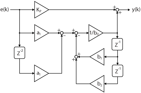
Once transformed into a difference equation, the resonant part yields:

$$y(k)={\displaystyle \frac{1}{b_0}[a_1\cdot e(k)-a_1\cdot e(k-2)-b_1\cdot y(k-1)-b_2\cdot y(k-2)]}$$

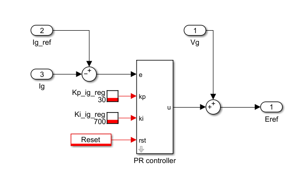
This difference equation can be easily used for generating run-time code. The corresponding block diagram is given below and can be easily replicated in Simulink or PLECS. A similar implementation is given in [2].

It is worth noting that the gains $b_0,b_1,$ and $b_2$ depend on the fundamental frequency ${\omega }_0$. As such, the PR controller can be made frequency-adaptive by calculating these coefficients at each execution step using frequency estimation methods such as a

SOGI-PLL for computing ${\omega }_0$.

Tuning and performance evaluation

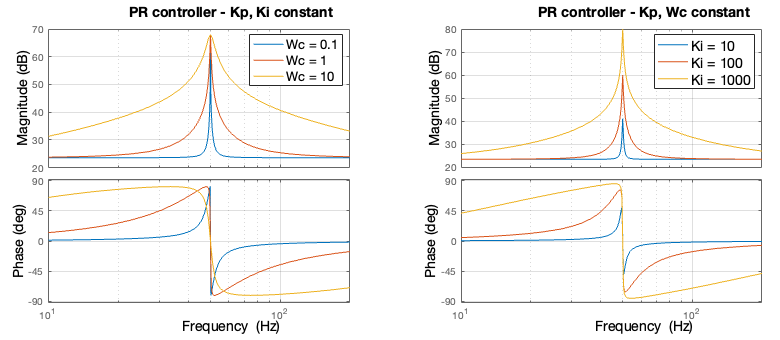
Proportional resonant controllers can be tuned relatively easily. In fact, three gains must be determined: $K_p,K_i,$ and ${\omega }_c$. The proportional gain $K_p$ defines the bandwidth and the phase margin in the same way as a PI controller. It can thus be tuned similarly, for example using the

magnitude optimum method. The parameters $K_i$ and ${\omega }_c$, on the other hand, define the “height” and “width” of the resonance peak. The following figures show the impact of these parameters on the controller transfer function. Further details regarding the tuning can notably be found in [3].

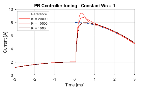
Additionally, the following figure illustrates the step response of the proposed resonant controller for various values of the resonant gain $K_i$.

Academic references

[1] D. N. Zmood and D. G. Holmes, “Stationary frame current regulation of PWM inverters with zero steady-state error,” in IEEE Trans. on Pow. Elec., Vol. 18, N°. 3, May 2003.

[2] R. Teodorescu, F. Blaabjerg, M. Liserre and P. C. Loh, “Proportional resonant controllers and filters for grid-connected voltage-source converters,” in IEE Proc. on Electr. Power Appl., Vol. 153, N°. 5, Sep. 2006.

[3] D. G. Holmes, T. A. Lipo, B. P. McGrath and W. Y. Kong, “Optimized Design of Stationary Frame Three Phase AC Current Regulators,” in IEEE Trans. on Pow. Elec., Nov. 2009.

B-Box / B-Board implementation

Simulink

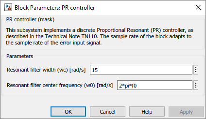
The Simulink model provided above contains a subsystem that uses the above-presented resonant controller implementation. This block can easily be integrated into any control algorithm. Besides, the provided dialog box offers simple configuration parameters.

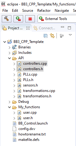
C/C++ code

Implementation example

#include "../API/controllers.h"
PrController mycontroller;   #resonant controller object
 
float Kp = 10.0;
float Ki = 500.0;
float w0 = TWO_PI*50.0;
float wc = 10.0;
 
tUserSafe UserInit(void)
{
    ConfigPrController(&mycontroller, Kp, Ki, w0, wc, SAMPLING_PERIOD);
    return SAFE;
}Code language: C++ (cpp)

tUserSafe UserInterrupt(void)
{
    //... some code
    Evsi = Vgrid + RunPrController(&mycontroller, Igrid_ref - Igrid);
    //... some code
    return SAFE;
}Code language: C++ (cpp)

Experimental results

In order to illustrate the performance of the proposed PR controller implementation, current control results are shown below. A current reference step is performed both in simulation (dark red) as well as using an experimental setup (light red). The following graphs show a comparison between both results :

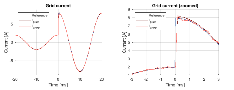
As it can be seen, the current matches the given reference in steady state. However, slight discrepancies between simulation and experimental results are observed due to harmonic distortions present on the grid.