Table of Contents
This technical note presents a possible implementation of a Rotor Field-Oriented Control (RFOC) of an Induction Machine (IM) with a squirrel cage.
First, the note introduces the general operating principles of the RFOC. Then, it explains how the stator’s electrical speed and position can be estimated from the mechanical speed of the rotor.
Finally, a practical control implementation is introduced, targeting the B-Box RCP or B-Board PRO with the ACG SDK on Simulink. Please note that imperix offers a ready-to-use motor drive system to develop and test motor control techniques. More details can be found in the Motor Testbench quick start guide (PN181).
General principles of Rotor Field-Oriented Control
The technical note TN111 introduces the principles of a Field-Oriented Control (FOC) for a Permanent Magnets Synchronous Machine (PMSM). In the case of an induction machine with a squirrel cage [1], the general idea is the same: the flux and torque are controlled independently in a Reference Rotating Frame (RRF) by – respectively – the d and q components of the stator current.
However, there are two key differences between a PMSM and an IM [2]: the rotor of the IM is mechanically not synchronous with the stator flux. Additionally, the IM does not have permanent magnets on the rotor: instead, the rotor is magnetized from the stator. Consequently, the FOC from the PMSM must be adapted to take these key differences into account.
Choice of the orientation
As mentioned above, the rotor is not necessarily rotating at the same speed as the stator (mechanically speaking). Therefore, unlike a PMSM (TN111), there are multiple ways to orient the RRF for an IM. Decoupled control of torque and flux quantities can be achieved by orienting the RRF on the stator, rotor, or air-gap fluxes [3]. In this note, Rotor Field-Oriented Control (RFOC) is chosen for its simplicity and higher torque dynamics [3].
In an induction machine, the rotor flux frequency is the sum of the mechanical and the slip frequencies [4]. The mechanical frequency is measurable but the slip must be estimated as explained in the RRF orientation section.
System-level modeling of a Rotor Field-Oriented Control
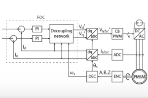
The independent control of \(I_{ds}\) and \(I_{qs}\) can consist of two PI regulators with a decoupling network, as any vector control strategy [1]. The FOC algorithm usually generates voltage references that a PWM modulator transforms into gating signals for a voltage source inverter. In this note, the rotor position measurement is derived from an incremental encoder. The figure below shows the complete block diagram of the implementation, with a carrier-based PWM modulator and an encoder/decoder module. Please note that space vector modulation could alternatively be used to improve the DC bus utilization.
 of an induction machine > RFOC_principle.png (Rotor Field-Oriented Control block diagram)")
All the speeds and angles are expressed as electrical quantities.
- \(\omega _m\) : the mechanical speed of the rotor (stationary reference frame)
- \(\omega _r\) : the speed of the rotor flux (stationary reference frame)
- \(\omega _s\) : the speed of the stator flux (stationary reference frame)
- \(\omega _{slip} = \omega _r – \omega _m\) : the speed of the rotor flux (rotor reference frame)
The corresponding angles are then obtained by integration.
Modeling of the induction machine
Now that the orientation of the RRF is chosen, a model of the machine can be established in this frame.
The equation of the stator circuit is [4]:
$$\displaystyle (1) \qquad \underline{V}_{dqs} = R_s \underline{I}_{dqs} + \frac{d \underline{\Psi}_{dqs}}{dt} + j \omega _r \underline{\Psi}_{dqs}$$
The equation of the rotor circuit is [4]:
$$\displaystyle (2) \qquad 0 = R_r \underline{I}_{dqr} + \frac{d \underline{\Psi}_{dqr}}{dt} + j (\omega _r – \omega _m)\underline{\Psi}_{dqr}$$
The fluxes are then linked to the currents [4] by:
$$\displaystyle (3) \qquad \underline{\Psi}_{dqs} = L_s \underline{I}_{dqs} + L_m \underline{I}_{dqr} \\ \quad \quad \quad \displaystyle (4) \qquad \underline{\Psi}_{dqr} = L_r \underline{I}_{dqr} + L_m \underline{I}_{dqs}$$
Finally, the torque is [4]:
$$\displaystyle (5) \qquad T_{em} = \frac{3}{2} p (\Psi _{ds} I_{qs} – \Psi _{qs} I_{ds})$$
In the literature [4], equations (1) – (4) are commonly used to establish an equivalent circuit of the machine in steady-state as presented in the figure below. Notice that the iron resistance is often neglected because I_fe is much smaller than the other currents.
 of an induction machine > equivalent_circuit.png (Steady-state equivalent circuit of a squirrel cage induction machine)")
| Parameter | Symbol |
|---|---|
| Stator resistance | \(R_s\) |
| Stator inductance | \(L_s\) |
| Stator leakage inductance | \(L_{\gamma s}\) |
| Mutual inductance | \(L_m\) |
| Parameter | Symbol |
|---|---|
| Rotor resistance * | \(R_r\) |
| Rotor inductance* | \(L_r\) |
| Rotor leakage inductance* | \(L_{\gamma r}\) |
| Iron resistance | \(R_{fe}\) |
* Rotor variables referred to the stator side
From (4), the rotor current can be expressed as:
$$\displaystyle (6) \qquad \underline{I} _{dqr} = \frac{1}{L_r} (\underline{\Psi} _{dqr} – L_m \underline{I}_{dqs})$$
In an induction machine with a squirrel cage, the rotor circuit is not accessible. Therefore, the rotor current \(\underline{I} _r\) cannot be measured and must be eliminated from the previous expressions.
By substituting (6) into (3), \(\underline{I} _r\) is removed from the stator flux expression:
$$\displaystyle (7) \qquad \underline{\Psi} _{dqs} = L_{\sigma}\underline{I} _{dqs} + \frac{L_m}{L_r} \underline{\Psi} _{dqr} \qquad \text{with} \space L_{\sigma} = L_s – \frac{L_m^2}{L_r}$$
In a similar way, \(\underline{I} _r\) is removed from the rotor circuit equation (2):
$$\displaystyle (8) \qquad \frac{d \underline{\Psi} _{dqr}}{dt} = \frac{L_m}{T_r} \underline{I} _{dqs} – \left(j (\omega _r – \omega _m) + \frac{1}{T_r}\right) \underline{\Psi} _{dqr} \qquad \text{with} \space T_r = \frac{L_r}{R_r}$$
Rotor flux control
The next step is to establish how to control the rotor flux. In an induction machine with a squirrel cage, there is no access to the rotor circuit and no permanent magnets. Therefore, the rotor must be magnetized from the stator.
Equation (8) suggests that the rotor flux can be controlled by the stator current. Assuming that the RRF is correctly aligned on the rotor flux, let us split equation (8) into its real and imaginary parts:
$$\displaystyle (9) \qquad \frac{d \Psi _r}{dt} = \frac{L_m}{T_r} I_{ds} – \frac{1}{T_r} \Psi _r \\ \displaystyle (10) \qquad 0 = \frac{L_m}{T_r} I_{qs} – (\omega _r – \omega _m) \Psi _r$$
From (9), the rotor flux is directly proportional to the d-axis stator current in steady-state:
$$\displaystyle (11) \qquad \Psi _r = L_m I_{ds}$$
Torque control
Once the rotor is magnetized, the machine can produce torque. Equation (5) describes the torque as a function of the stator flux and current. Assuming that the RRF is correctly aligned on the rotor flux, equation (7) becomes:
$$(12) \qquad \left\{ \begin{array}{ll} \displaystyle \Psi _{ds} &= L_{\sigma} I_{ds} + \frac{L_m}{L_r} \Psi _r \\ \displaystyle \Psi _{qs} &= L_{\sigma} I_{qs} \end{array}\right.$$
By injecting (12) into (5), the torque can be expressed as a function of the rotor flux and the q-axis current component.
$$\displaystyle (13) \qquad T_{em} = \frac{3}{2} p \frac{L_m}{L_r} \Psi _r I_{qs}$$
If the rotor flux is kept constant, the torque is directly proportional to the q-axis component of the stator current.
Current controller for Rotor Field-Oriented Control
As explained in the previous section, the rotor flux and the torque are directly proportional to the d and q components of the stator current. Therefore, they can be controlled using a stator current controller.
The stator circuit is described by (1). By injecting (7) into (1), it is possible to replace the stator flux with the rotor flux.
$$\displaystyle (14) \qquad \underline{V}_{dqs} = R_s \underline{I}_{dqs} + L_{\sigma} \frac{d \underline{I}_{dqs}}{dt} + j \omega _r L_{\sigma} \underline{I}_{dqs} + \frac{L_m}{L_r} \frac{d \underline{\Psi}_{dqr}}{dt} + j \omega _r \frac{L_m}{L_r} \underline{\Psi}_{dqr}$$
Assuming that the RRF is correctly aligned on the rotor flux, the real and imaginary parts of (14) are:
$$(15) \qquad \left\{ \begin{array}{ll} \displaystyle V_{ds} &= R_s I_{ds} + L_{\sigma} \cfrac{d I_{ds}}{dt} – \omega _r L_{\sigma} I_{qs} + \cfrac{L_m}{L_r} \cfrac{d \Psi_{r}}{dt} \\ V_{qs} &= R_s I_{qs} + L_{\sigma} \cfrac{d I_{qs}}{dt} + \omega _r L_{\sigma} I_{ds} + \omega _r \cfrac{L_m}{L_r} \Psi_{r} \end{array}\right.$$
The first two terms of the equations in (15) express the link between the voltage and current at the stator. This relation can be reformulated as a transfer function: it is the same on both axes:
$$(16) \qquad H_d(s) = H_q(s) = \frac{I_{s}(s)}{V_{s}(s)} = \frac{1/R_s}{1 + s \space L_{\sigma}/R_s} = \frac{K_1}{1 + s \space T_1}$$
The transfer function in (16) expresses how the current reacts to a change in the voltage input generated by the inverter. Thus, with the help of a PI controller, it is possible to control the currents at the stator. The PI tuning is addressed in the following section.
The third term of the equations in (15) corresponds to the coupling of the axes. TN106 explains how a decoupling network can be used to allow truly independent control of the d and q axes.
The last term corresponds to the effect of the rotor flux on the stator circuit. As explained previously, it is desirable to keep the rotor flux constant to simplify the torque control. Therefore, since \(d \Psi _r/dt = 0\), only the q-axis is affected by the rotor flux. The term \(\omega_r \frac{L_m}{L_r} \Psi_r\) can be computed by the control and added to the q-axis voltage reference.
Tuning of the controller
As covered in [5], the magnitude optimum criterion is a suitable way to tune a PI when the transfer function of the plant is of the same form as in (16). The controller parameters are:
$$(17) \qquad \left\{ \begin{array}{ll} T_n &= T_1\\ T_i &= 2 K_1 T_d \\ K_p &= T_n / T_i \\ K_i &= 1 / T_i\end{array}\right.$$
The parameter \(T_d\) represents the sum of all the small delays in the system. The product note PN142 explains how to determine the total delay of the system.
Current references
To use the machine under nominal conditions, the rotor flux should be nominal.
From (11), the rotor flux is set by the d-axis current reference:
$$\displaystyle (18) \qquad I_{ds}^* = \frac{\Psi _r^*}{L_m} = \frac{\Psi _{rn}}{L_m} = I_{dsn}$$
The q-axis current reference is then derived from (13):
$$\displaystyle (19) \qquad I_{qs}^* = \cfrac{T_{em}^*}{\cfrac{3}{2} p \cfrac{L_m}{L_r} \Psi _r}$$
There is however a minor inconvenience at startup: the machine cannot be magnetized instantaneously. Thus, when the flux \(\Psi_r\) is still building up, the current consumption will be large according to (19).
If the current consumption at startup is a concern, the flux can be assumed to be constant and equal to its nominal value. In this case, the machine cannot produce the torque reference because the rotor flux is overestimated. However, it happens only during the startup transient. Therefore, the impact on the control performances is minimal.
Calculation of the nominal d-axis current
If the nominal rotor flux is unknown in (18), the nominal d-axis current can be calculated from the nominal voltage, the nominal current, and the equivalent circuit of the machine.
From the equivalent circuit:
$$\displaystyle (20) \qquad \underline{V}_{s} = R_s \underline{I}_s + j \omega _s (L_s – L_m) \underline{I}_s + \underline{V}_m$$
Taking \(\arg( \underline{V}_s) = 0 \,\text{rad}\) as the reference phase, the real and imaginary parts of \(\underline{V}_m\) are then:
$$(21) \qquad \left\{ \begin{array}{l} \displaystyle \text{Re}\{\underline{V}_m\} = V_s – R_s I_s \cos\phi + \omega _s (L_s – L_m) I_s \sin\phi \\ \\ \displaystyle \text{Im}\{ \underline{V}_m\} = – R_s I_s \sin\phi – \omega _s (L_s – L_m) I_s \cos\phi \end{array}\right.$$
with \(\cos \phi\) the power factor of the machine.
If the RRF is correctly aligned on the rotor flux, the magnetizing current is equal to the d-axis component of the stator current. Assuming that the iron losses can be neglected:
$$\displaystyle (22) \qquad V_m = \sqrt{\text{Re}\{\space \underline{V}_m\}^2 + \text{Im}\{\space \underline{V}_m\}^2} = \omega _s L_m I_m = \omega _s L_m \frac{I_{ds}}{\sqrt{2}}$$
From (22), the d-axis current is then:
$$\displaystyle (23) \qquad I_{ds} = \frac{\sqrt{2} V_m}{\omega _s L_m}$$
The nominal d-axis stator current is found by solving equations (21) to (23) using the nominal voltage \(V_{sn}\) and current \(I_{sn}\) of the IM. The power factor is usually available in the machine datasheet.
Dynamic saturation
The output of the current controller is a voltage reference to generate with the voltage source inverter (VSI). However, the maximal output voltage of the VSI is limited by the DC bus voltage. In the RRF, this saturation limit corresponds to a circle of radius \(V_{dc}/\sqrt{3}\). The figure on the right illustrates the situation in one quadrant: as long as the reference voltage is inside the circle, it can be generated by the VSI.
The current controller must take the saturation of the VSI into account with a proper anti-windup strategy. Since there is one PI controller per axis, saturation limits should be defined on a per-axis basis.
 of an induction machine > Dynamic_saturation.png (Saturation limits in the rotating reference frame)")
A first option would be to use the same limits for both axes. In the figure above, \(\underline{V}_1^*\) is the extreme case where the full DC bus voltage is used and where both components have the same saturation limits. In this case, the limits are set to \(\pm V_{dc}/\sqrt{6}\). While this solution is simple to implement, it does not use the full potential of the DC bus: \(\underline{V}_2^*\) and \(\underline{V}_3^*\) are both valid references even if they are outside the \(\pm V_{dc}/\sqrt{6}\) boundaries.
A second option is then to compute the saturation limits dynamically. According to (19), the IM cannot produce a torque if the rotor is not magnetized beforehand. Therefore, the d-axis PI current controller should have priority. With this logic, \(V_{ds}\) can use whatever it needs from the DC bus voltage, and \(V_{qs}\) takes whatever is left:
$$(24) \qquad \left\{ \begin{array}{ll} |V_{ds}| &\leq \cfrac{V_{dc}}{\sqrt{3}} \\ \\ |V_{qs}| &\leq \sqrt{\cfrac{V_{dc}^2}{3} – V_{ds}^2} \end{array}\right.$$
The saturation limits are then expressed as:
$$(25) \qquad \left\{ \begin{array}{ll} V_{ds,sat} &= \pm \cfrac{V_{dc}}{\sqrt{3}} \\ \\ V_{qs,sat} &= \pm \sqrt{\cfrac{V_{dc}^2}{3} – \min\left(V_{ds}^2,\cfrac{V_{dc}^2}{3}\right)} \end{array}\right.$$
RRF orientation for Rotor Field-Oriented Control
In the previous sections, the RRF was assumed to be oriented on the rotor flux. The question is then: how to orient the RRF correctly? To align the RRF on the rotor flux, the position of the flux must be known. In [6] and [7], the authors present a FOC variant called Indirect Field-Oriented Control (IFOC). This method is indirect because the rotor flux is estimated from the model of the machine.
Let us assume that the RRF is indeed oriented on the rotor flux. In this case, from (9), the rotor flux can be estimated from the d-axis current:
$$ (26) \qquad \Psi _r = \cfrac{L_m}{s \space T_r + 1} I_{ds}$$
According to (10), the slip frequency is calculated from the q-axis current:
$$(27) \qquad \omega _{slip} = \omega _r – \omega _m = \frac{L_m}{T_r \Psi _r} I_{qs}$$
Then, by re-arranging the terms in (27):
$$(28) \qquad \omega _r = \omega _m + \omega _{slip}$$
The rotor mechanical speed \(\omega_m\) is either measured or estimated. Finally, the position of the RRF is obtained from the stator electrical speed:
$$(29) \qquad \theta _r = \int _0 ^t \omega _r \space dt $$
B-Box / B-Board implementation of Rotor Field-Oriented Control
Software resources
The code example is ready for use with the Motor Testbench. It includes:
- an induction machine with a Rotor Field-Oriented Control, and a speed controller
- a permanent magnets synchronous machine to load the IM. The Field-Oriented Control of the PMSM is presented in TN111.
Rotor flux angle estimation
The indirect method to orient the rotating reference frame uses the equations (26-29) and its implementation is shown below. It computes the rotor flux angle \(\theta_r\) used to transform the stator currents in the dq frame.
 of an induction machine > image2021-2-24_11-16-45.png (Rotor flux angle estimation Simulink model)")
Stator current controller
The stator current control in the rotor RRF is shown below. The decoupling network uses the rotor flux speed \(\omega_r\) estimated by the indirect method above. The d-axis current reference is computed with equation (23) and imposes a nominal rotor flux. The q-axis current reference is derived from the torque reference, using equation (19). Finally, dynamic saturation limits of the d- and q-axis regulators are computed using equation (25).
 of an induction machine > image2021-2-24_12-14-1.png (Stator current controller Simulink model)")
Speed controller
The speed controller is the same as in TN114 and computes the necessary torque reference for the cascaded torque (i.e. current) controller. In the present implementation, the integral term of the speed controller (outer loop) is kept at reset when the current controller (inner loop) hits its saturation to avoid accumulating large errors.
Experimental results of Rotor Field-Oriented Control
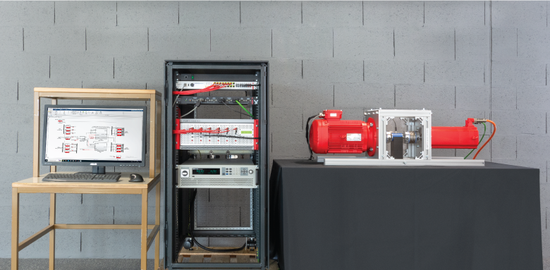
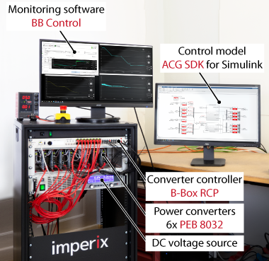
The experimental setup consists of an induction machine and a permanent magnet synchronous machine (PMSM). The PMSM is used to apply a load torque on the IM. Each machine is supplied by a voltage source inverter made of 3x PEB 8032 phase-leg modules . The control code of each machine is implemented on Simulink, using the ACG SDK library, and both algorithms run on a single B-Box RCP controller.
The following experimental results are all exported from the datalogger of the BB Control software (now replaced by Cockpit) and post-processed using MATLAB.
Machine parameters
The parameters of the induction machine are given in the table below. The PMSM (Control Techniques 115UMC300CACAA) was chosen to operate under the same nominal conditions.
| Model: Leroy-Somer 2P LSES 100L 3kW | |||
| Parameter | Symbol | Value | Unit |
| Rated power | \(P_n\) | 3 | kW |
| Pole pairs | \(p\) | 1 | – |
| Rated phase voltage | \(V_{sn}\) | 230 | V |
| Rated phase current (wye-connected) | \(I_{sn}\) | 6.1 | A |
| Rated mechanical speed | \(\Omega_n\) | 2870 | rpm |
| Rated torque | \(T_{em,n}\) | 9.95 | Nm |
| Rated power factor | \(\cos \phi\) | 0.88 | – |
| Stator resistance | \(R_s\) | 1.5 | Ω |
| Stator inductance | \(L_s\) | 307 | mH |
| Rotor resistance* | \(R_r\) | 1.4 | Ω |
| Rotor inductance* | \(L_r\) | 313 | mH |
| Mutual inductance | \(L_m\) | 295 | mH |
| Moment of inertia (IM only) | \(J_m\) | 0.0036 | kg m2 |
* The rotor variables are referred to the stator side.
Speed tracking performance of the Rotor Field-Oriented Control
The tracking performance of the speed controller was validated experimentally by applying a speed reference step from 0 to 2870 rpm. At the same time, the PMSM was applying a load torque proportional to the speed. In the end, the IM was operating at nominal speed and with a 9.5 Nm load in steady-state.
Since the speed controller is tuned using the symmetrical optimum criterion [8], a rate limiter was applied to the speed reference to limit the overshoot. The use of a rate limiter is detailed in TN114. During the experimental validation, the acceleration was limited to 2870 rpm/s. This way, the IM can reach its nominal speed in ~1s with practically no overshoot.
The experimental results are presented below. Notice that, at the very beginning, the rotor does not move immediately, leading to poor tracking performance. This behavior is due to the absence of magnetization, as detailed in the next section.
 of an induction machine > speed-torque-tracking.png (Speed tracking and load torque)")
Since this is an induction machine, the mechanical speed of the rotor \(\omega_m\) is slower than the rotor flux \(\omega_r\) under load (see below on the left). Let us recall the definition of the relative slip [4]:
$$(30) \qquad s = \frac{\omega _r – \omega_m}{\omega_r}$$
At startup, the slip is equal to 1 because the rotor is at a standstill. However, the machine quickly moves to a stable operating point with a low slip as illustrated below (right). In steady-state, the relative slip is approximately \(s\approx 0.023\).
 of an induction machine > slip-tracking-performances.png (Rotor mechanical speed and slip)")
Disturbance rejection
It was shown previously that the speed controller can track the speed reference. However, it should also be capable of rejecting a disturbance (i.e. a load torque).
To verify the disturbance rejection, the speed of the IM was ramped up to 2870 rpm under no load. Then, a step from 0 to 9.5Nm was applied by the PMSM (see below on the left). It can be observed in the figure below (right) that the current controller managed, simultaneously, to keep the flux constant (through \(I_{ds}\)) and adapt the torque (through \(I_{qs}\)). This is made possible by the independent control of the d and q axis stator currents. Notice that the speed controller reaches its upper saturation limit which was set to 110% of the nominal torque.
 of an induction machine > torque-current-distrubance-rejection.png (Motor torque and current tracking)")
At the same time, the speed controller must adapt the torque reference to maintain the rotor mechanical speed constant. Since the slip increases with the load (see below on the right), the frequency of the rotor flux must be increased to keep the mechanical speed constant. During the transient, the mechanical speed drops ~5.2% below the reference and it takes ~150 ms to recover from the load step.
 of an induction machine > slip-distrubance-rejection.png (Rotor speed and slip)")
Comparison between Rotor Field-Oriented Control and V/f control
As mentioned in the theoretical part of this technical note, the RFOC belongs to the family of vector control methods. However, V/f control of an induction machine (TN138) presents a simpler scalar control method called V/f control. What is the point of implementing a (rather complex) RFOC instead of a V/f algorithm? To answer this question, the same induction machine was used to undergo the same tests in both the V/f and RFOC technical notes.
Speed tracking
In the figure below, the experimental speed tracking performance of the V/f and RFOC are superimposed for comparison purposes.
The tracking performances of the V/f and RFOC are indistinguishable in most of the speed ranges. The only significant difference lies in the low-speed region, here the V/f has a dead zone, whereas the RFOC has no such limitations. Remember that, once the IM is magnetized, the RFOC can operate at any speed without distortions. Therefore, the V/f control is a compelling option as long as low-speed operation is not required.
 of an induction machine > tracking-speed-vs-torque.png (Speed tracking and load torque comparison)")
Even if the RFOC and the closed-loop V/f maintain the rotor at the same mechanical speed, the slip is larger with the V/f. This is due to a slight difference in the magnetization of the machine: with the V/f, the norm of the stator flux is maintained constant and equal to its nominal value. Thus, the norm of the rotor flux should also stay constant. However, when considering this flux in the rotor flux-oriented RRF, only the d-axis component magnetizes the machine. Since the V/f is only a scalar method, there is no explicit control of the d-axis component of the rotor flux.
Conversely, the RFOC does have explicit control of this d-axis component. Therefore, the RFOC maintains the d-axis component of the rotor flux to its nominal value instead of the norm of the vector. The slight difference in the rotor flux leads to a different torque-slip characteristic for each method, thus, a different slip under the same load.
According to the experimental results, under a load of 95.5% of the nominal torque, the slip is ~0.023 with the RFOC and ~0.027 with the closed-loop V/f. Theoretically, the lower the slip, the better, because the machine operates farther from its breakdown slip [4]. However, this is a concern only if the IM must operate at very high torque, close to its breakdown torque.
 of an induction machine > tracking-slip-frequency_v2.png (Rotor mechanical speed and slip comparison)")
Disturbance rejection
In the figure below, the experimental disturbance rejection performance of the V/f and RFOC are superimposed for comparison purposes.
There is a fundamental difference in the slip estimation (see below on the right) between the two methods: on the one hand, the RFOC estimates the slip from the model of the IM. Thus, the estimation is fairly accurate even during fast transients. On the other hand, the slip estimation from the V/f method relies on the PI of the speed controller (see the speed tracking section in the V/f control of an induction machine (TN138)). It means that, if the slip changes abruptly due to a sudden variation of the load, the slip estimation will change slowly through the integral action of the PI controller. Experimentally, the closed-loop V/f takes ~1750 ms to recover from the disturbance – nearly 12 times longer than the RFOC (~150 ms). This is a significant performance difference between the two methods.
 of an induction machine > rejection-slip.png (Roto mechanical speed and slip disturbance rejection)")
Academic references
[1] B. Robyns, B. François, P. Degobert, J.P. Hautier, “Vector Control of Induction Machines”, Springer, 2012.
[2] Nguyen Phung Quang, Jörg-Andreas Dittrich, “Vector Control of Three-Phase AC Machines”, Springer, 2015, ISBN 978-3-662-46914-9
[3] E. Y. Y. Ho and P. C. Sen, “Decoupling control of induction motor drives,” in IEEE Transactions on Industrial Electronics, vol. 35, no. 2, pp. 253-262, May 1988
[4] Slobodan N. Vukosavic, “Electrical Machines”, Springer, 2013.
[5] Karl J. Åström and Tore Hägglund, “Advanced PID Control”, 1995.
[6] A. K. Akkarapaka and D. Singh, “The IFOC based speed control of induction motor fed by a high performance Z-source inverter,” 2014 International Conference on Renewable Energy Research and Application (ICRERA), Milwaukee, WI, 2014, pp. 539-543.
[7] I. Ferdiansyah, L. P. S. Raharja, D. S. Yanaratri and E. Purwanto, “Design of PID Controllers for Speed Control of Three Phase Induction Motor Based on Direct-Axis Current (Id) Coordinate Using IFOC,” 2019 4th International Conference on Information Technology, Information Systems and Electrical Engineering (ICITISEE), Yogyakarta, Indonesia, 2019, pp. 369-372.
[8] Slobodan N. Vukosavić ,”Digital Control of Electrical Drives”, Springer, 2007, ISBN 978-0-387-25985-7