Finite control set MPC for a voltage-controlled inverter

This article introduces an example of Finite Control Set Model Predictive Control (FCS-MPC) for an LCL-filtered voltage-controlled inverter. The proposed control implementation is derived from [1], with an extension to minimize the output common-mode current. This is notably relevant when an EMC filter is required, such as when the inverter is connected to the grid (instead of a passive load).

After the introduction to the MPC working principle and plant modeling, the control algorithm is described and two implementations are provided: a full-CPU implementation, as well as an FPGA-based version. Both versions are validated experimentally and briefly discussed.

Working principle

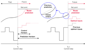
The idea behind any MPC implementation can be summarized as follows: if the behavior of the plant can be predicted, it is possible to select the best control input based on estimated forecasts. Therefore, given a set of possible control inputs (or candidates), the MPC includes two steps: the prediction, for each candidate, of the future state (based on the plant model), and then the selection of the best candidate.

The plant behavior is most often expressed as a linear state-space representation $\dot{x}=Ax+Bu$, from which a discretized state-space model $x_{k+1}=A_d{x}_k+B_d{u}_k$ can be derived through exact discretization. The selection of the best candidate then requires the formulation of an objective (or cost) function $g$, in which the minimized quantities may be adapted depending on the desired dynamics.

With a finite set of candidates, the future state is usually estimated for each of them. From this forecast, the associated cost can be easily derived, such that the best candidate (lowest cost) can be identified at the end of the process. When the output can be any value within a given interval (infinite set of candidates), both steps are considered at once: the cost function is expressed as a function of the state-space model and then minimized through an exact optimization or using a solver.

With a suitable plant model, it is theoretically possible to predict states for a large number of sampling periods and sequentially apply the candidates corresponding to the best sequence. However, because of unavoidable disturbances, noise, and potential modeling approximations, only the first element of the sequence is usually applied, and the best sequence is computed again at the next time step to improve the control robustness. The number of anticipated values is called the horizon $N$. In this example, the horizon is kept to 1.

A further introduction to MPC is given in

Discrete plant model

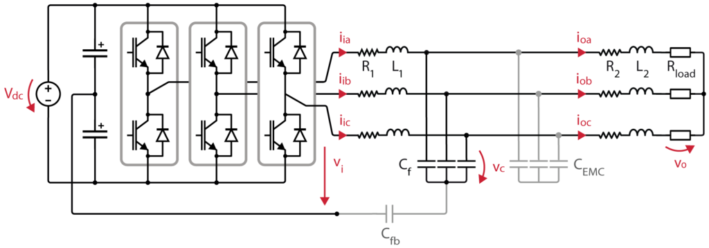
The considered circuit is depicted in Fig. 1. Components marked in gray are ignored for the moment. They will be considered when introducing the extension in the next section.

The equations describing the plant dynamics are as follows:

$$\begin{array}{rlrlrl}\frac{d{i}_i}{dt}& =\frac{1}{L_1}(v_i-R_1{i}_i-v_c)& \frac{d{v}_c}{dt}& =\frac{i_i-i_o}{C_f}& \frac{d{i}_o}{dt}& =\frac{1}{L_2}(v_c-R_2{i}_o-v_o)\end{array}$$

where $i_i$ and $i_o$ are the inverter and load currents, and $v_o$, $v_c$, $v_i$ the load, capacitor and inverter voltages. These variables are represented by their complex vectors in the αβ frame. For instance, the inverter-side current in the αβ-frame is:

$$i_i=i_{i\alpha }+j{i}_{i\beta }=\frac{2}{3}(i_{ia}+a\cdot i_{ib}+a^2\cdot i_{ic})$$

where $a=e^{j2\pi /3}$. The inverter-side voltage can then be expressed in terms of the switching states of each phase $S_a$, $S_b$, and $S_c$:

$$v_i=\frac{2}{3}{V}_{dc}(S_a+a{S}_b+a^2{S}_c)$$

Since the load current $i_o$ can be measured, there’s no need to use the third equation (system dynamics), allowing the reduction of the prediction model, represented in a state-space form as:

$$\dot{x}=Ax(t)+Bu(t)=\left[\begin{array}{cc}-\frac{R1}{L1}& -\frac{1}{L1}\\ \frac{1}{C_f}& 0\end{array}\right]\left[\begin{array}{c}{i}_i\\ v_c\end{array}\right]+\left[\begin{array}{cc}\frac{1}{L1}& 0\\ 0& -\frac{1}{C_f}\end{array}\right]\left[\begin{array}{c}{v}_i\\ i_o\end{array}\right]$$

where $x\left(t\right)={\left[i_i{v}_c\right]}^T$ and $u\left(t\right)={\left[v_i{i}_o\right]}^T$ are the state and input vectors, respectively.

The discretized state-space model of the system is then:

$$\left[\begin{array}{c}{i}_{i,k+1}\\ v_{c,k+1}\end{array}\right]=A_d\left[\begin{array}{c}{i}_{i,k}\\ v_{c,k}\end{array}\right]+B_d\left[\begin{array}{c}{v}_{i,k}\\ i_{o,k}\end{array}\right]=e_{}^{A{T}_s}\left[\begin{array}{c}{i}_{i,k}\\ v_{c,k}\end{array}\right]+{\int }_0^{T_s}{e}^{A𝜏}Bd𝜏\left[\begin{array}{c}{v}_{i,k}\\ i_{o,k}\end{array}\right]$$

where $A_d$ and $B_d$ are obtained through exact discretization. This can be typically achieved during code generation using the expm Matlab command, which computes the matrix exponential using a scaling and squaring algorithm with a Pade approximation [3] :

% Symbolic Math Toolbox required
Ad = expm(A*Ts); 
Bd = (integral(@(Ts) expm(A.*Ts),0,Ts, 'ArrayValued', true))*B;Code language: Matlab (matlab)

Cost function for finite control set MPC

Reference tracking

The considered control aims at controlling the line-to-line voltages across the $C_f$ capacitors. Since the capacitor voltage dynamics are mainly determined by the inverter-side currents, the control method proposed in [1] consists of delaying the desired voltage reference and transforming it into a current reference. Doing so, authors assume that voltages and currents are designed at grid frequency, and are thus slowly varying in comparison to the controller’s sampling frequency (i.e. $i_{o,k+2}^{\ast }\approx i_{o,k}$ and $v_{i,k+2}^{\ast }\approx v_{i,k+1}$). Although this assumption could be questioned for $v_{i,k}^{\ast }$, the corresponding implementation shows good performance.

Using the discrete state-space model and the coefficients of matrices $A_d$ and $B_d$, the prediction of the capacitors voltage in the αβ-frame is:

$$v_{c,k+3}=A_{d,10}{i}_{i,k+2}+A_{d,11}{v}_{c,k+2}+B_{d,10}{v}_{i,k+2}+B_{d,11}{i}_{o,k+2}$$

The inverter-side current reference can be derived as:

$$i_{i,k+2}^{\star }=\frac{v_{c,k+3}^{\star }-A_{d,11}{v}_{c,k+2}-B_{d,10}{v}_{i,k+2}-B_{d,11}{i}_{o,k+2}}{A_{d,10}}$$

where $i_{i,k+2}$, $v_{c,k+2}$ are forecasts obtained by application of the system’s model and $i_{o,k+2}^{\ast }\approx i_{o,k}$ and $v_{i,k+2}^{\ast }\approx v_{i,k+1}$ are the best available estimates for $i_{o,k+2}$ and $v_{i,k+2}$.

In this example, the objective function uses a quadratic norm and is designed only for current tracking:

$$g={(i_{i\alpha ,k+2}^{\star }-i_{i\alpha ,k+2}^{})}^2+{(i_{i\beta ,k+2}^{\star }-i_{i\beta ,k+2}^{})}^2$$

where $i_{\alpha ,k+2}^{\star }$, $i_{\beta ,k+2}^{\star }$ and $i_{\alpha ,k+2}$, $i_{\beta ,k+2}$ are the current reference and prediction at sampling instant $k+2$.

Common mode current minimization

Besides the reference tracking strategy of [1], this example proposes to leverage the remaining degree of freedom to reduce the common mode current at the inverter output. This has several benefits, namely the possibility to use the inverter with an EMC filter – often required when connected to the grid – and the reduction of the maximal peak current in the inverter modules.

To this aim, the circuit of Fig. 1 is slightly modified and gray-marked components are now considered. A $C_{fb}$ feedback capacitor is added, creating a feedback path between the midpoint of the capacitive filter and the DC bus midpoint. An EMC filter is also added and can be modelized by an additional $C_{EMC}$ capacitive filter.

In differential mode, the system derived in the previous section still holds, except that $C_f+C_{\text{EMC}}$ should be considered instead of $C_f$, because both capacitive filters are now seen in parallel. The feedback path does not affect the differential-mode behavior.

In common mode, the obtained model (not explicitly derived here) is almost the same as in differential mode, where the only difference is that ${(1/C_f+1/C_{fb})}^{-1}$ should now be considered instead of $C_f$. This defines the common-mode model $x_{0,k+1}=A_d^0{x}_{0,k}+B_d^0{u}_{0,k}$ and makes it possible to forecast the common-mode voltage $v_{i0,k+2}$ and current $i_{i0,k+2}$.

The common-mode current $i_{i0,k+2}$ is then penalized through an additional term appended to the cost function, leading to:

$$g={(i_{i\alpha ,k+2}^{\star }-i_{i\alpha ,k+2}^{})}^2+{(i_{i\beta ,k+2}^{\star }-i_{i\beta ,k+2}^{})}^2+K\cdot i_{i0,k+2}^2$$

where $K=50$ has shown good performance.

Algorithm implementation

The control routine of the proposed Finite Control Set MPC algorithm can be synthesized as follows:

1. Get the measured quantities (ii, vc, io, Vdc) from the ADC at instant k;
2. Considering that the control routine computation time corresponds to one period and that the new optimal state will thus be applied just before the next iteration, get an estimate of ii and vc at instant k+1;
3. For each candidate:
   • Get an estimate of ii and vc at instant k+2;
   • Get an estimate of ii_ref at instant k+2;
   • Compute the candidate’s cost;
4. Select the best candidate (lowest cost) and apply it.

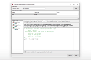
The algorithm is implemented in C and embedded within the Simulink environment via a S-Function block. More information about S-Functions can be found in

float simulate_state(
    const float sw[3],
    float Vdc,
    float IO[2],
    float Vref[3],
    float ii_k1[3],
    float vc_k1[3],
    float Ad[2][2],
    float Bd[2][2],
    float Ad0[2][2],
    float Bd0[2][2],
    int mode) {

    float vi_k1[3];
    float ii_k2[3];
    float vc_k2[3];
    float iiref_k2[3];

    float cost = 0;

    // 2nd-step calculations for the alpha/beta-components
    for(int i=0;i<2;i++) {
        vi_k1[i] = Vdc*sw[i];

        ii_k2[i] = Ad[0][0]*ii_k1[i] + Ad[0][1]*vc_k1[i] + Bd[0][0]*vi_k1[i] + Bd[0][1]*IO[i];
        vc_k2[i] = Ad[1][0]*ii_k1[i] + Ad[1][1]*vc_k1[i] + Bd[1][0]*vi_k1[i] + Bd[1][1]*IO[i];

        iiref_k2[i] = (Vref[i] - Ad[1][1]*vc_k2[i] - Bd[1][0]*vi_k1[i] - Bd[1][1]*IO[i]) / Ad[1][0];

        cost += (iiref_k2[i]-ii_k2[i])*(iiref_k2[i]-ii_k2[i]);
    }

    // 2nd-step calculations for the 0-component
    if (mode==1) {
        vi_k1[2] = Vdc*sw[2]-Vdc/2;

        ii_k2[2] = Ad0[0][0]*ii_k1[2] + Ad0[0][1]*vc_k1[2] + Bd0[0][0]*vi_k1[2] + Bd0[0][1]*IO[2];
    
        cost += 50*ii_k2[2]*ii_k2[2];
    }

    return cost;
}

// (...)

void MPC_Outputs_wrapper(const real32_T *Vdc_ptr,
                         const real32_T *ii_ptr,
                         const real32_T *vc_ptr,
                         const real32_T *io_ptr,
                         const real32_T *vref_ptr,
                         const real32_T *Ad_ptr,
                         const real32_T *Bd_ptr,
                         const real32_T *Ad0_ptr,
                         const real32_T *Bd0_ptr,
                         const int32_T *mode_ptr,
                         uint32_T *out) {

    float Vdc = *Vdc_ptr;
    float *IM = (float*)ii_ptr;
    float *V = (float*)vc_ptr;
    float *IO = (float*)io_ptr;
    float *Vref = (float*)vref_ptr;
    float Ad[2][2] = {{Ad_ptr[0], Ad_ptr[2]},{Ad_ptr[1], Ad_ptr[3]}};
    float Bd[2][2] = {{Bd_ptr[0], Bd_ptr[2]},{Bd_ptr[1], Bd_ptr[3]}};
    float Ad0[2][2] = {{Ad0_ptr[0], Ad0_ptr[2]},{Ad0_ptr[1], Ad0_ptr[3]}};
    float Bd0[2][2] = {{Bd0_ptr[0], Bd0_ptr[2]},{Bd0_ptr[1], Bd0_ptr[3]}};
    int mode = *mode_ptr;
    
    // constants
    const float _1_3 = 0.33333333;
    const float _2_3 = 0.66666667;
    const float _sqrt3_3 = 0.57735027;

    // possible switching states
    // leg_a = LSB, leg_c = MSB
    const unsigned int states[8] = {0b000, 0b001, 0b011, 0b010, 0b110, 0b100, 0b101, 0b111};

    // normalized alpha/beta/0-components at the output of the inverter
    // corresponding to the switching states of states[7]
    const float sw[8][3] =
        {{0, 0, 0}, {_2_3, 0, _1_3}, {_1_3, _sqrt3_3, _2_3}, {-_1_3, _sqrt3_3, _1_3}, {-_2_3, 0, _2_3}, {-_1_3, -_sqrt3_3, _1_3}, {_1_3, -_sqrt3_3, _2_3}, {0, 0, 1}};

    // current state
    static int x_k = 0;

    // start of 1st step
    float vi_k[3];
    float ii_k1[3];
    float vc_k1[3];

    // 1st-step calculations for the alpha/beta-components
    for(int i=0;i<2;i++) {
        vi_k[i] = Vdc*sw[x_k][i];
    }

    for(int i=0;i<2;i++) {
        ii_k1[i] = Ad[0][0]*IM[i] + Ad[0][1]*V[i] + Bd[0][0]*vi_k[i] + Bd[0][1]*IO[i];
        vc_k1[i] = Ad[1][0]*IM[i] + Ad[1][1]*V[i] + Bd[1][0]*vi_k[i] + Bd[1][1]*IO[i];
    }

    // 1st-step calculations for the 0-component
    if (mode==1) {
        vi_k[2] = Vdc*sw[x_k][2]-Vdc/2;
    
        ii_k1[2] = Ad0[0][0]*IM[2] + Ad0[0][1]*V[2] + Bd0[0][0]*vi_k[2] + Bd0[0][1]*IO[2];
        vc_k1[2] = Ad0[1][0]*IM[2] + Ad0[1][1]*V[2] + Bd0[1][0]*vi_k[2] + Bd0[1][1]*IO[2];
    }

    // start of 2nd step
    float g;
    float min_g = 1e18;
    int min_ind = 0;

    // simulation of all possible states and identification of the optimal one
    for (int i=0; i<8; i++) {
        g = simulate_state(sw[i], Vdc, IO, Vref, ii_k1, vc_k1, Ad, Bd, Ad0, Bd0, mode);

        if (g < min_g) {
            min_g = g;
            min_ind = i;
        }
    }

    // update of state and out
    x_k = min_ind;
    *out = states[x_k];
}Code language: C++ (cpp)

Experimental setup

The suggested setup, used to validate the proposed finite control set MPC implementation, includes the following imperix products :

• Programmable controller (B-Box RCP)
• ACG SDK toolbox for automated generation of the controller code from Simulink
• 3x PEB8024 modules (mounted e.g. in type A or type C rack)
• 1x passive filters rack or:
  • 6x 2.5mH inductors (L1, L2)
  • 3x 10µF capacitors (Cf)
  • 3x 3.3uF capacitors (EMC)
• 3x DIN 800V voltage sensors
• 3x DIN 50A current sensors

and additional components :

• 1x DC power supply
• 1x 1uF capacitors (Cfb)
• 3x 30Ω power resistors

The system parameters of the chosen case study are given in the following table :

To prevent any damage, the hardware protection thresholds of the B-Box RCP front panel must be correctly configured. The suggested values are gathered in the table below. More information can be found in

CPU implementation

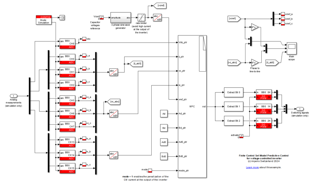
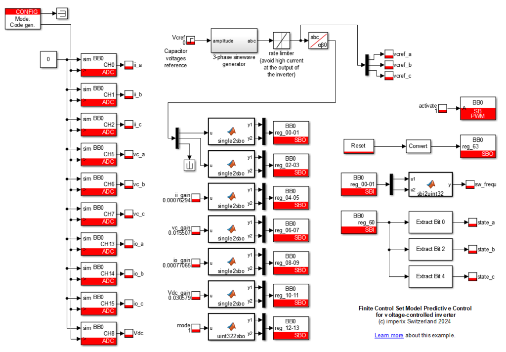
Simulink model

The Simulink model can be downloaded here below. It uses the imperix ACG SDK and can both simulate the behavior of the system (offline simulation) and generate code for real-time execution on a B-Box RCP.

Validation results

To assess the transient performance of the control, the capacitor voltage reference is set to 250V at t=0, 100V at t=50ms, and subsequently to 330V at t=100ms.

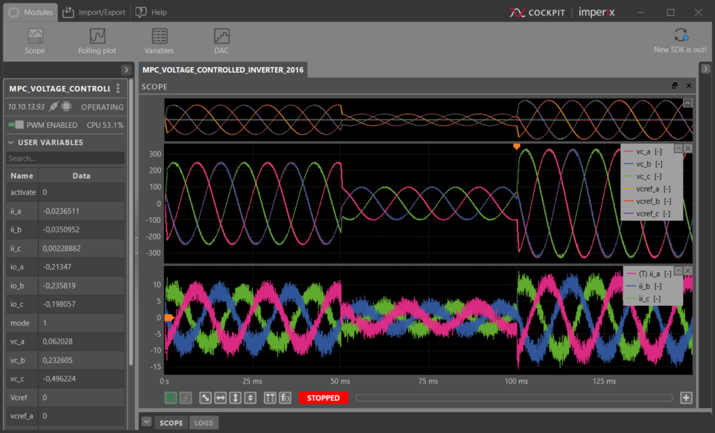
The control algorithm correctly tracks the reference step change, confirming its proper operation.

FPGA implementation

Vivado project

The Vivado project can be downloaded here below, along with the corresponding Simulink model and additional files. The C files used to generate the IP via Vitis HLS, as described in

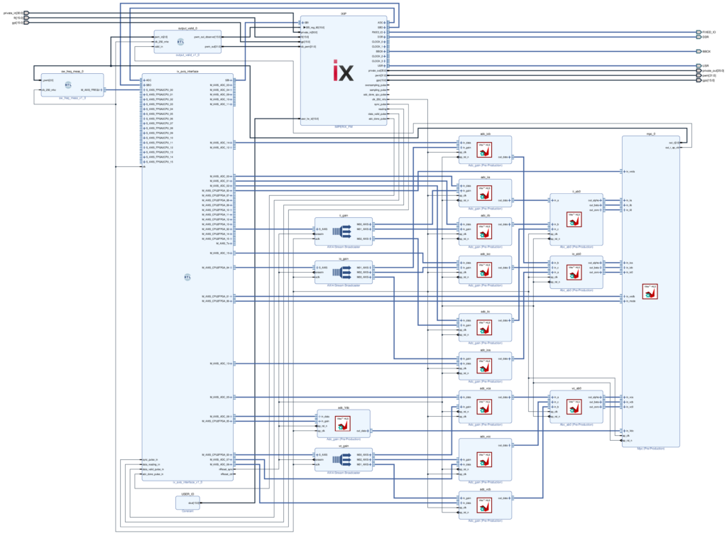
The data is propagating as AXIS streams, ensuring that the Finite Control Set MPC algorithm is executed at the sampling frequency. The AXIS broadcasters are receiving the gains from the Simulink model and dispatching them to the adc_gain blocks to apply them to the raw data. The αβ-frame projection is then obtained at the output of the abc_ab0 blocks, before being fed to the mpc.

The 3-bit output of the Finite Control Set MPC is cast within a 32-bit vector in the output_valid block and provided to the IX IP to be applied. The sw_frequ_meas block measures the actual switching frequency of the first phase with a 1-kHz resolution.

The common-mode current minimization can be ignored by setting the mode parameter to 0 (instead of 1, by default), resulting in a reference tracking in the αβ-frame only.

Simulink model

The Simulink model required to use Cockpit and communicate with the FPGA is available in the .zip archive of the previous section. Additional information about the communication between the CPU and the FPGA can be found in

The switching frequency (computed in the FPGA) is available as sw_frequ. This signal is updated every 1ms and has a 1-kHz resolution. The switching states are available as state_{a,b,c}. They require the CPU interrupt frequency to be equal to the sampling frequency to be shown correctly.

Validation results

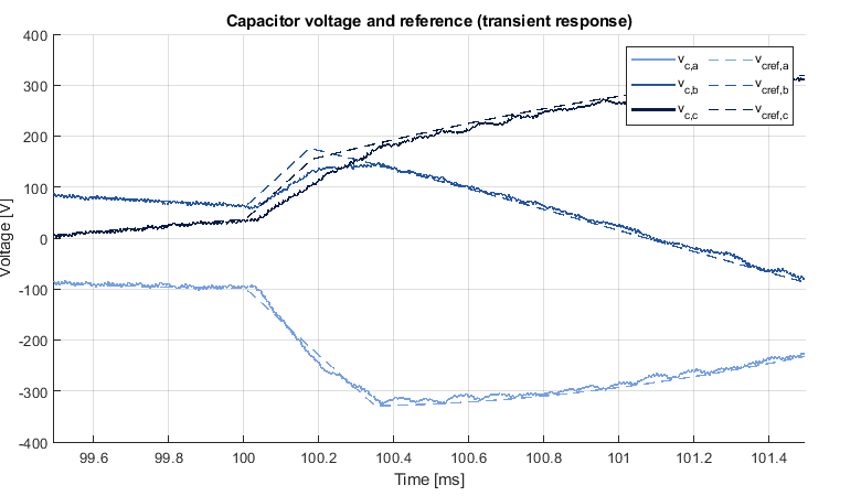
To assess the transient performance of the control, the capacitor voltage reference is set to 250V at t=0, 100V at t=50ms, and subsequently to 330V at t=100ms.

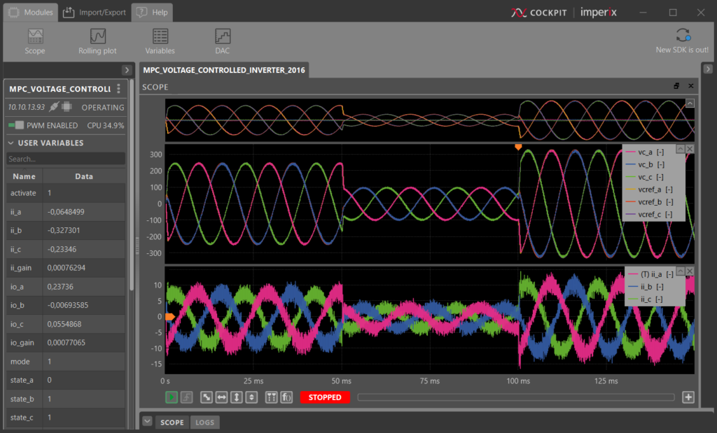
The control algorithm correctly tracks the reference step change, confirming its proper operation.

A zoom on the corresponding transient response is shown in Fig. 7, where the reference voltage amplitude is increased from 100V to 330V at t=100ms. The maximal reference slope is limited in the software to avoid high currents in the inverter modules. The rate limit is set to ±330V/ms. Even with this limitation, the setpoint is reached in less than 2% of the fundamental period (400us vs. 20ms).

Conclusion

The validation results of Fig. 3 and 6 show that the behavior of the Finite Control Set MPC is the same for the CPU and FPGA versions of the controller, both executed with a sampling frequency of 100kHz. The transient response is also particularly fast, as shown in Fig. 7, where the setpoint is reached in less than 2% of the fundamental period.

Furthermore, the provided results show that the CPU-based implementation is exactly equivalent to its FPGA-based counterpart. As such, engineers are truly free to choose the implementation option of their liking. On one hand, using the FPGA for the execution of the Finite Control Set MPC algorithms could be preferred as it spares CPU resources for other tasks. On the other hand, the CPU-based approach is significantly quicker and easier to implement and validate.

Finally, it is also worth noting that further investigations on that topic (not displayed here) revealed that increasing the sampling frequency doesn’t necessarily reduce the current ripple, or significantly improve the control dynamics. Indeed, although simulation results are slightly better at 150kHz, laboratory tests done at 120 and 150kHz showed that this is not the case in practice.

References

[1] H. A. Young, V. A. Marin, C. Pesce, and J. Rodriguez, “Simple Finite Control Set Model Predictive Control of Grid-Forming Inverters With LCL Filters,” in IEEE Access, April 2020.

[2] J. Rodríguez and P. Cortés, Predictive Control of Power Converters and Electrical Drives, Wiley, 2012.

[3] A. Al-Mohy and N. Higham, “A New Scaling and Squaring Algorithm for the Matrix Exponential”, in SIAM Journal on Matrix Analysis and Applications, Vol. 31, 2009.

[4] T. Dragičević, “Model Predictive Control of Power Converters for Robust and Fast Operation of AC Microgrids,” in IEEE Trans. of Power Electronics, July 2018.

[5] P. Cortes, J. Rodriguez, C. Silva and A. Flores, “Delay Compensation in Model Predictive Current Control of a Three-Phase Inverter,” in IEEE Trans. of Power Electronics, Feb. 2012.

[6] P. Karamanakos, E. Liegmann, T. Geyer and R. Kennel, “Model Predictive Control of Power Electronic Systems: Methods, Results, and Challenges,” in IEEE Open Journal of Industry Applications, Vol. 1, 2020.