Table of Contents
The operation of a grid-tied power converter (such as the 3-phases PV inverter) requires that the control software implements a grid synchronization technique. One well-known approach consists in using a three-phase PLL to project the AC grid quantities into a synchronous rotating reference frame. The PLL algorithm is usually executed on the CPU of the controller, but it can be alternatively offloaded to the FPGA.
Besides the obvious benefit of offloading the CPU, the execution of the synchronization algorithm on an FPGA also allows for a much shorter control latency, ultimately enabling full-FPGA ultra-fast control loops, as presented in FPGA-based inverter control.
This note will cover the implementation of a simple PLL-based grid synchronization algorithm that is suitable for being executed on the FPGA of the B-Box and B-Board controllers.
Overview of the grid synchronization module
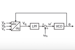
The grid synchronization algorithm implemented in FPGA is based on a conventional DQ-PLL, similar to the CPU implementation presented in the TN103. The PLL consists of an abc-to-dq transformation (used as a phase detector), a PI regulator (used as a low-pass filter), and a wrapping integrator (used as a voltage-controlled oscillator). The grid synchronization module also projects the measured grid current into the synchronously rotating reference frame, so the projected dq components can be used by the FPGA-based dq current control module.
The following sections detail how to pack that algorithm into the FPGA IP shown below, using both High-Level Synthesis tools Vitis HLS and Model Composer. That IP uses AXI4-Stream inputs and outputs to be compatible with other IPs developed on other pages, as well as with Xilinx IP cores for Vivado.
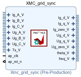
Further details on integrating that IP into the FPGA are presented on the High-Level Synthesis page. A complete converter control algorithm that uses that IP is presented in FPGA-based converter control.
FPGA implementation of the PLL with Model Composer (Simulink)
The sources of the grid synchronization module developed with Xilinx Model Composer can be downloaded below. To generate a Vivado IP from this model using Model Composer’s automatic code generation please refer to the introduction to Model Composer.
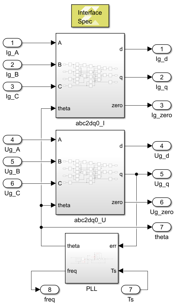
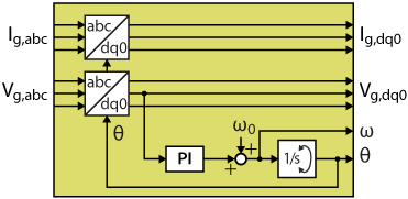
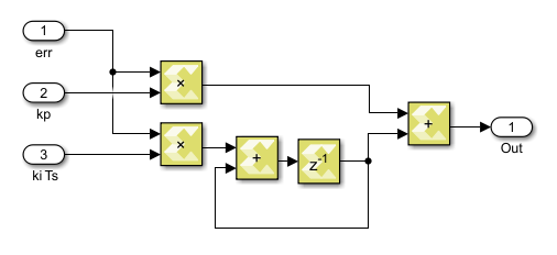
Basically, this module includes two abc-to-dq0 transformations and one PLL. The PI controller used within the PLL block is based on the implementation presented in the Model Composer introduction.
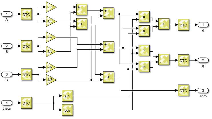
The abc-to-dq0 transformation simply implements the mathematical formulae introduced in abc to dq0. In both Vitis HLS and Model Composer, fixed-point types are used to represent the intermediary results. Specifically, all the angles (radians) are represented with fix16_12 and the other quantities are represented with fix32_16. The main reason is that floating-point trigonometric functions are computationally heavy and cannot meet the timing requirement. As a side benefit, using fixed-point operations also improves the resource usage and latency of the other operations (multiplications and additions). Nevertheless, to ensure compatibility with other modules, the inputs and outputs of the coordinate transformations are converted into floating-point types.
As seen later in the section “Precision of the fixed-point approach”, the loss of precision caused by the use of fix16_12 numbers for representing angles is negligible in practice (lost in the noise), although small differences can be seen in simulation.
In Model Composer, there is no need to specify the data types or implementation methods, and the software will automatically call the HLS math library during code generation.
Testbench of the Model Composer implementation
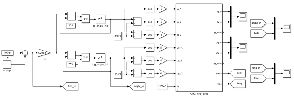
One main advantage of Model Composer over Vitis HLS is that test benches can be easily run directly from within Simulink. The testbench generates 50 Hz three-phase voltages and currents and passes them as inputs to the developed PLL. To test the frequency tracking of the PLL, the input frequency is stepped to 52 Hz at t=0.02s.
Mathematically, the inputs of the testbench are:
| Voltages | Currents | Time |
| $$\begin{aligned} &U_{a}=311\cdot\sin(2\pi f nT_{s}) \\ &U_{b}=311\cdot\sin(2\pi f nT_{s} – 2\pi/3) \\ &U_{c}=311\cdot\sin(2\pi f nT_{s} + 2\pi/3)\end{aligned}$$ | $$\begin{aligned}&I_{a}=5\cdot\sin(2\pi f nT_{s}) \\ &I_{b}=5\cdot\sin(2\pi f nT_{s} – 2\pi/3) \\ &I_{c}=5\cdot\sin(2\pi f nT_{s} + 2\pi/3) \end{aligned}$$ | $$\begin{aligned}&n=0,1,2,…,1999 \\ &T_s=50\,\text{µs} \\ &f=\begin{cases}50 & n\leqslant 400 \\ 55 & n>400 \end{cases} \end{aligned} $$ |
After running the Simulink-based simulation, the inputs and outputs can be exported to the MATLAB workspace and plotted, as shown below.
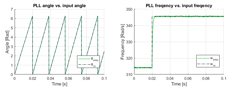
The simulation results are identical to the Vitis HLS approach shown below.
FPGA implementation of the PLL with Vitis HLS (C++)
The full Vitis HLS implementation of the PLL can be downloaded below and the main lines of code are given for reference.
The code is divided into the following functions:
void abc2dq0(float A, float B, float C, float wt, float& d, float& q, float& zero)
Transforms the three-phase AC quantitiesA,B,Cintod,q,zerocomponents, using the reference frame anglewt.void pll(float Ugq, float Ts, float& theta, float& freq)
Runs a discrete PI controller (with discretization periodTs) using the alignment errorUgqand updates the output angle (theta, in rad) and frequency (freq, in rad/s). The controller parameterspll_kpandpll_ki, as well as the central frequencyw0, are defined in thegrid_sync.hfile.void vitis_grid_sync( ... )
Runs the PLL algorithm on the grid quantitiesin_Igabcandin_Ugabcto compute the grid angle (out_theta) and frequency (out_freq), as well as the components of the grid quantities in the dq synchronous reference frame.
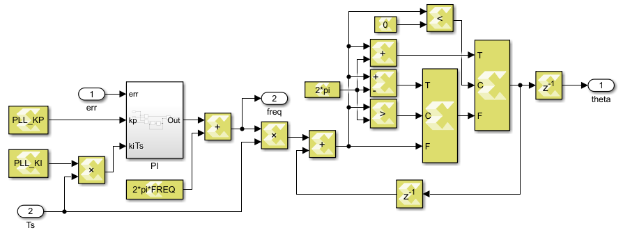
The wrapping integrator is implemented using the code below, to avoid the modulo-based wrapping used in the CPU version. Since this approach only uses switches and comparators, it is much better suited to an FPGA implementation than the resource-consuming modulo function.
const float theta_max = 6.283185307179586;
const float theta_min = 0;

static float wrapping_accum = 0;
#pragma HLS RESET variable=wrapping_accum

wrapping_accum += Ts * w;

if(wrapping_accum > theta_max)
{
  wrapping_accum -= theta_max;
}
else if(wrapping_accum < theta_min)
{
  wrapping_accum += theta_max;
}Code language: C++ (cpp)
Note that the vitis_grid_sync method uses AXI4-Stream interfaces to be compatible with the other functions developed for the TN147. More information about Vitis HLS can be found in the introduction to Vitis HLS, notably on how to create an IP out of the provided code to run the algorithm on the FPGA of a B-Box or B-Board controller.
#pragma HLS inline is a directive that removes a function as a separate entity in the hierarchy and enables optimization with surrounding operations. It’s recommended to use this directive when defining a child function in Vitis HLS. Look at pragma HLS inline (xilinx.com) to see more details.Testbench of the Vitis HLS implementation
To validate the Vitis HLS implementation, a testbench can be built using the code provided below.
Here, the exact same testbench as with Model Composer (same inputs) is implemented. The C Simulation tool of Vitis HLS is used to run the testbench. The input and output data are stored in “Vitis_grid_sync\solution1\csim\build” and can be plotted for comparison (e.g. with MATLAB). The results are shown below:
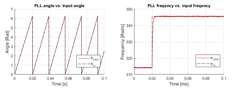
The simulation results show that the angle and frequency estimated by the PLL follow the input accurately, although some noise with relatively low amplitude can be observed on the PLL frequency. This matter will be addressed in a dedicated section, and the performance will also be compared to the already validated CPU-based model provided with the imperix blockset.
Precision of the fixed-point approach
As introduced before, fix16_12 fixed-point angles are used inside the coordinate transformation blocks since floating-point trigonometric functions cannot meet the timing requirements. This conversion to fixed-point inevitably results in a loss of precision, which can be seen as “noise” in the testbench results.
For sake of validation, if the angle is represented with fix32_28 instead of fix16_12, all the visible estimation “noise” disappears completely, as illustrated below. Unfortunately, the implementation cannot meet the timing requirements if fix32_28 is used.
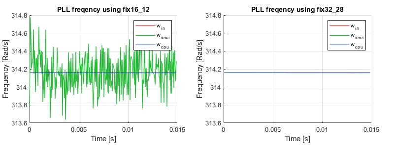
A floating-point implementation (cpu) is also shown for reference.
Representing angles with fix16_12 numbers allows for an absolute angular resolution of \(1/2^{12}\approx 0.00024 \,\text{rad}\), which corresponds to a precision of 0.004%. As for the other variables, using fix32_16 numbers gives an absolute resolution of \(1/2^{12}\approx 15 \,\text{µV}\) or \(\text{µA}\).
The simulation testbench results showed that the resulting error on the estimated frequency is at most 0.2%, which is considered acceptable in real systems, where the measurement accuracy is rather in the 1% range.
Usecase example
The developed FPGA PLL is used for grid synchronization in the FPGA ctrl of a grid-tied 3-phase inverter.