

Table of Contents
This article addresses possible implementations for a discrete PI controller and provides general insight into PI tuning strategies. It also includes practical implementations for digital control, on Simulink, PLECS, and C/C++.
General principles
PI controllers certainly represent the most intuitive and widespread form of closed-loop (feedback) control. As such, they are frequently implemented in both continuous (analog) and discrete (digital) domains. This is notably due to their simple structure and implementation, relying on two steps:
- The controller computes the difference between the desired setpoint and the measured variable. This value is considered an error.
- The PI controller computes a control action proportional to this error (proportional part) and ensures the process output matches the setpoint at steady state (integral part).
PI controller structure
Controller type
Imperix generally uses PI controllers rather than PID controllers to avoid the complexity and instability issues associated with the derivative action. More precisely, the high-frequency gain of the derivative action can indeed cause amplification of measurement noise, which is undesirable. Also, PID controllers generally bring only little improvement when paired with first-order systems (which are very common in power electronics) [1].
Controller structure
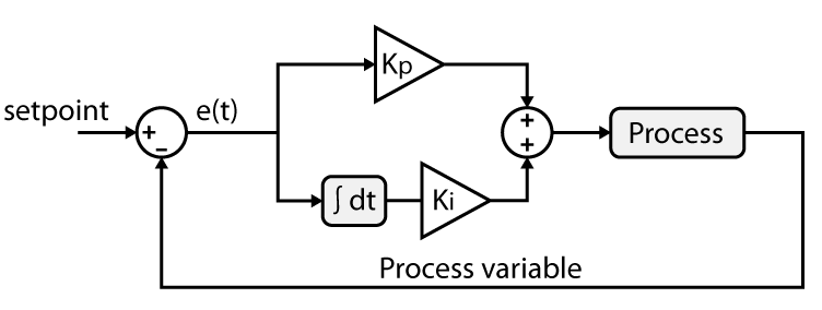
PI controllers can be implemented in parallel (non-interacting), series (interacting), or mixed form [2]. This article focuses on the parallel structure of PI controllers, which fully decouples the proportional and integral terms and makes manual tuning easier. The block diagram below describes the implementation of a parallel PI controller.
Digital implementation
The well-known continuous-time transfer function of a PI controller, given below, should be discretized for implementation in a digital controller.
$$ (1) \quad C(s) = k_p + \frac{k_i}{s}$$
Here, \(k_p\) and \(k_i\) are the proportional and integral gains of the controller, respectively.
Usually, when discretizing a continuous function for a control system, the main goals are to preserve its frequency behavior and stability characteristics. To this end, several possible discretization strategies exist, amongst which the three most common are Forward Euler, Backward Euler, and Tustin [3]. Discussing these methods is outside the scope of this article. Nonetheless, the benefits and drawbacks of each method can be summarized as follows [4]:
- Forward Euler: Simple and computationally efficient, but suffers from poor stability.
$$ (2) \quad s = \frac{z-1}{T_s} $$ - Backward Euler: Unconditionally stable, but more computationally intensive than Forward Euler.
$$ (3) \quad s = \frac{z-1}{T_sz} $$ - Tustin: Preserves continuous-time stability and offers superior frequency accuracy compared to Euler methods, at the cost of higher implementation complexity.
$$ (4) \quad s = \frac{2}{T_s}\frac{z-1}{z+1} $$
Where \(T_s\) is the discrete time interval.
The following section focuses on the forward Euler method. A similar approach applies to the other two methods mentioned above.
The discretized equation of the PI controller using the forward Euler method then results in the following equation:
$$ (5) \quad C(z) = \frac{Y(z)}{E(z)} = K_p + K_i T_s \frac{1}{z-1} $$
In the end, as the objective is to implement a PI controller inside a digital control system, the discretized PI controller can be translated into the following difference equations:
$$ (6) \quad \begin{aligned}
& y(k) = P(k) + I(k) = k_p \cdot e(k) + I(k)\\
& I(k) = I(k-1) + k_i \cdot T_s \cdot e(k-1) \\
\end{aligned}$$
Where \(e(k)\) is the error input (the difference between the targeted setpoint and the measured value), and \(y(k)\) is the output of the PI controller.
PI controller tuning strategies
Tuning PI controllers should consider trade-offs among tracking performance, perturbation rejection, measurement noise, and other practical aspects. Many strategies exist, such as Ziegler-Nichols, loop shaping, optimization, pole placement, etc.
This section further details a popular optimization method, the magnitude optimum (MO), often chosen for its good trade-off between simplicity and performance. This strategy aims for a good response to setpoint changes, but it may offer limited disturbance rejection. In power electronics, MO is frequently applied to first-order systems, such as current control loops. Alternatively, the symmetric optimum (SO) criterion can be used when the focus is set on disturbance rejection. In power electronics, this is often applied to cascaded voltage control loops (speed, position, DC-link voltage…) on top of an inner loop that was already tuned by magnitude optimum. These two criteria are well presented in [5].
The objective of the MO tuning method is to design a controller so that the overall system output (controller + plant) exactly and instantaneously reproduces its input. That is, the overall system’s transfer function is unity at all frequencies [5]. This assumes an ideal controller that perfectly compensates for plant dynamics, which is impossible in practice. Instead, applying the MO criterion translates to achieving a response curve that is as flat and as close to unity as possible over the widest possible bandwidth.
To derive the magnitude optimum’s parameters, a first-order plant model is considered, described in the Laplace domain, by the equation below:
$$ (7) \quad P_1(s) = \frac{K_1}{1+s T_1}$$
The PI controller transfer function is rewritten as:
$$ (8) \quad C(s) = \frac{1+sT_n}{sT_i}$$
The actuator delay is also taken into account and approximated by a first-order model as well:
$$ (9) \quad D(s) = e^{(-sT_{d,tot})} \approx \frac{1}{1+s T_{d,tot}}$$
The generic formulas for MO shown below can then be used to tune PI controllers [5].
$$ (10) \quad \begin{aligned}
&T_n = T_1\\
&T_i = 2 K_1 T_{d,tot}
\end{aligned}$$
For the symmetric optimum, the generic formulas are shown below [5]
$$ (11) \quad \begin{aligned}
&T_n = 4 T_{d,tot}\\
&T_i = 8 K_1 T_{d,tot}^2/T_1
\end{aligned}$$
Rewriting (8) as in (1) results in the following equations for \(K_p\) and \(K_i\):
$$ (12) \quad \begin{aligned}
&K_p = T_n /T_i\\
&K_i = 1 / T_i
\end{aligned}$$
The parameter \(T_{d,tot}\) represents the sum of all the delays in the system (from the data acquisition to the control output). For a practical example of PI controller tuning, see: PI-based current control.
PI controller configuration
Several techniques can improve the closed-loop behavior. For instance, anti-windup strategies, setpoint weighting, feedforward, and cascaded control can improve conventional PI controllers [1]. A strategy to limit integrator windup is given in the section below.
Integrator wind-up and anti-windup methods
When the control system must adjust to a large disturbance or setpoint variation, the integrator accumulates a significant error (wind-up) during the transient phase. This can also happen when a physical variable reaches its limits (for example, in a switched-mode power supply, the duty cycle is usually bounded between 0 and 1). So when the output finally reaches the reference, the large value accumulated by the integral term creates a significant, undesired output overshoot.
To eliminate this unwanted effect, anti-windup algorithms can be implemented. Several techniques are commonly used, such as [1]:
- Conditional integration
- Back calculation
- Automatic reset
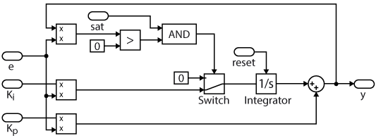
The illustration below details the conditional integration algorithm, which will disable the integrator when the following two conditions are fulfilled:
- The PI controller output saturates.
- The control and error signals have the same sign (When they don’t, the integrator can help push the controller’s output out of saturation).
Reset
While the control task is not actively running (during system initialization, shutdown, or when transitioning between control modes for instance) it is often necessary to prevent the integrator from accumulating error. PI controllers commonly provide an external reset mechanism to address this. As part of the imperix blockset, the Core state block outputs the appropriate reset signal, which can be directly connected to the external reset input of PI controllers. Obviously, this signal is only relevant in an experimental setup and is not useful in simulation.
B-Box / B-Board implementation
Simulink and PLECS
The (discrete) PID controller blocks in Simulink and PLECS can be used to implement control algorithms. Please refer to TN109 for configuration examples of both Simulink and PLECS PI controllers.
C/C++ code
The imperix IDE provides numerous pre-written and pre-optimized functions. Controllers such as P, PI, PID, and PR are already available and can be found in the controllers.h/.cpp files.
As for all controllers, PI controllers are based on:
- A pseudo-object
PIDcontroller, which contains pre-computed parameters as well as state variables. - A configuration function, meant to be called during
UserInit(), namedConfigPIDController(). - A run-time function meant to be called during the user-level ISR, such as
UserInterrupt(), namedRunPIController().
Note that this C/C++ implementation of the PI controller is slightly different from the one described above. More information on this implementation is available in [5].

References
[1] A. Visioli, “Practical PID Control”, 2006
[2] Karl J. Åström and Tore Hägglund, “Advanced PID Control”, 1995
[3] Buso, S. and Mattavelli, P., “Digital Control in Power Electronics: Second Edition”, 2015
[4] Franklin, G.F., Powell, J. and D.Workman, M.L., “Digital Control of Dynamic Systems”, 1998
[5] J. W. Umland and M. Safiuddin, “Magnitude and symmetric optimum criterion for the design of linear control systems: what is it and how does it compare with the others?,” in IEEE Trans. on Industry Applications, May-June 1990.
 By Jessy Ançay • May 8, 2023 • TN109

 By Jonathan Orsinger • March 30, 2021 • AN006