PI based current control

This technical note presents a conventional PI controller-based current control strategy, using a buck converter as example. The developed example may be employed as an introduction to imperix’s toolset and as a reference model to perform first tests on new equipment.

Many applications, such as motor drive, battery chargers and grid-connected inverters require current control, or regulation. This article will considers the current control of a buck converter operating in continuous conduction. Practical information on how to set-up such a system is available in PN119. Details about the component sizing as a well as continuous vs. discontinuous conduction are also given in TN100.

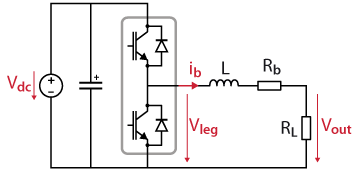
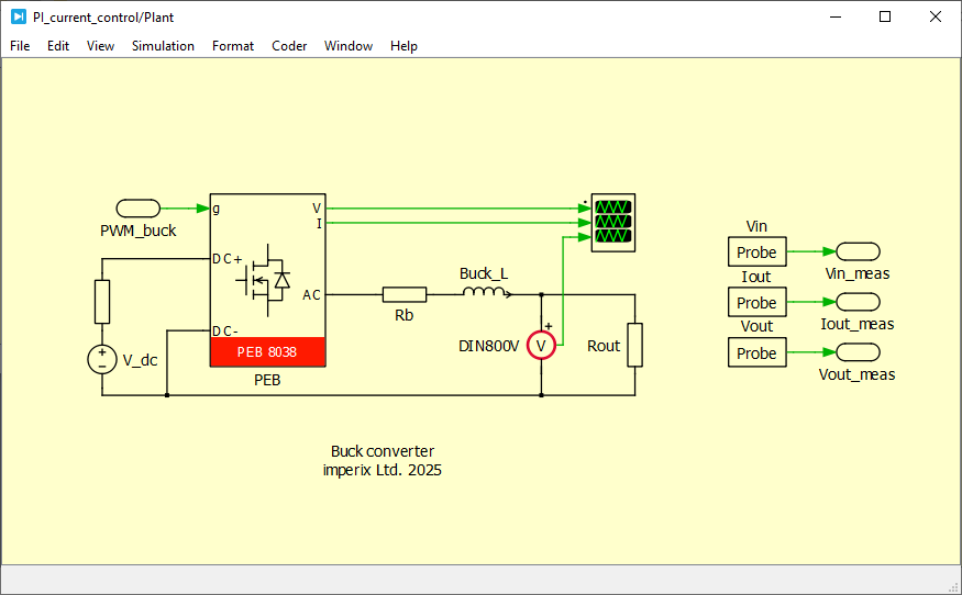
The simplified schematic of the considered system is presented below. \(R_{b}\) is the equivalent series resistance of the inductor, otherwise designated as \(L\). A passive load is considered, represented by \(R_{L}\).

Elementary principles of current control

Current control is generally implemented by leveraging the inductive energy stored inside an inductor. In other words, leveraging the fact that the current flowing through an inductor is a function of the voltage across its terminals:

$$I= \frac{1}{L}\int_{}^{}(V_{1}-V_{2})dt$$

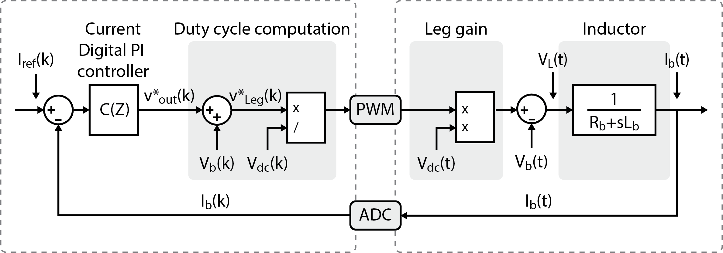
In a buck converter, the output current is therefore controllable thanks to the difference between the converter voltage \(V_{leg}\) and the measured output voltage \(V_{out}\). In this case, \(V_{L}=V_{leg}-V_{out}\) is the input variable (the control variable), and \(i_{b}\) is the output variable.

Translated into the Laplace domain this yields the first order transfer function below:

$$\cfrac{I_L(s)}{V_L(s)} = \cfrac{1}{sL+R_{b}}$$

Performing a simple substitution, the well-known expression of a first order system can be retrieved:

$$P_1(s) = \displaystyle\frac{K_1}{1+s T_1} \qquad \text{with} \qquad \begin{cases}K_1 = 1/R_b \\ T_1 = L_b/R_b \end{cases}$$

The plant model transfer function being of the first order, it can then be controlled with a PI controller with zero steady-state error when tracking reference steps [2].

PI controller tuning

In most cases, it is desired to tune current control for tracking performance rather than for perturbation rejection. In other words, bandwidth is preferred over stability or robustness. In this case, a common criteria for tuning the PI controller parameters is the so-called “magnitude optimum” criteria. This sets:

More information on controller tuning is given in TN105.

Considering the buck converter’s transfer function, this yields:

$$K_p = \cfrac{L}{2T_{d,tot}} \quad \quad K_i = \cfrac{R_b}{2T_{d,tot}}$$

Where \(T_{d,tot}\) represents the total control delay, which can be considered as the sum of two terms:

1. The control delay \(T_{d,ctrl}\), corresponding to the delay between the sampling instant and the instant, at which the duty-cycle is updated within the PWM modulator. This is mostly the algorithm computation time.
2. The modulator delay \(T_{d,\text{PWM}}\), corresponding to the average delay between the duty-cycle update (i.e. the moment at which it is latched by the modulator) and the resulting change at the output.

In the present case, the sampling phase is set to \(\phi_s = 0.5\) to ensure sampling in the middle of the current ripple (with a triangular carrier for PWM). The cycle delay is shorter than half a control period since the control algorithm is very light, leading to a control delay of \(T_{d,ctrl}=T_s/2\). Finally, the triangular carrier with a single-rate update leads to a modulator delay of \(T_{d,\text{PWM}}=T_s/2\). In total, the delay is therefore one complete sampling period \(T_{d,tot}=T_s\).

More information on these delay and how they can be identified is given in TN142.

Numerically, considering a inductor value of 2.2mH with 0.033\(\Omega\) of series resistance (example from imperix’s passive filter box), the controller parameters become:

$$K_p = \cfrac{2.2\,\text{mH}}{2\times 50\,\text{µs}}=22\,\Omega \quad \quad K_i = \cfrac{0.033\,\Omega}{2\times 50\,\text{µs}}=330 \,\Omega\,\text{s}^{-1}$$

Feed-forward for buck converter current control

As described above, the current controller is therefore responsible for producing the necessary voltage across the inductor. Indeed, the considered plant is exclusively constituted by \(L\) and \(R_{b}\).

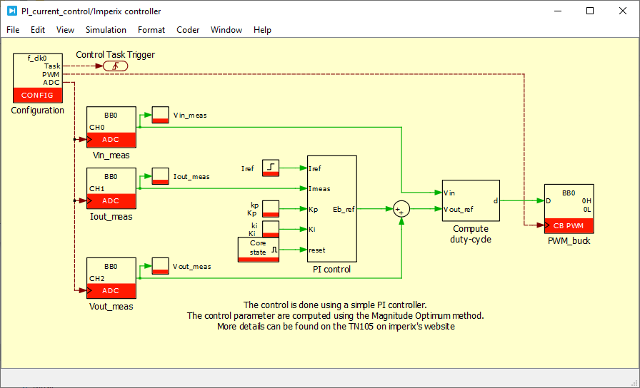
Therefore, as shown in Fig.2, the voltage that must be produced by the buck converter (reference voltage \(V^*_{leg}\)) is constituted by the sum of the measured load voltage \(V_{out}\) and the current controller output. In other words:

$$V^*_{leg} = V_{PI}+V_{out}$$

In this case, \(V_{out}\) is said to be feedforwarded to the controller output.

Interestingly, if \(V_{out}\) wasn’t used a a feed-forward term, the integral term of the current controller would naturally add up and compensate for that voltage. However, this integral action takes time and therefore cannot help reject rapid changes to the load conditions (e.g. load step). For this reason, feedforwarding the load-side voltage is generally favorable to current control performance.

On the other hand, when this load-side voltage measurement is of poor quality (e.g. noisy, or presenting a sensitivity error), feedforwarding can be rather detrimental. In such a case, the feedfoward signal rather represents an additional perturbation, which the current control must reject.

In the end, the benefits of voltage feedwording at the output of a current controller must therefore be evaluated on a case-by-case basis as a function of the quality of that feedforward signal. Filtering the signal before feedforwarding is also always possible, but with inevitable sacrifices on the corresponding bandwidth.

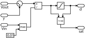
Duty cycle computation

Based on the computed reference voltage \(V^*_{leg}\), the duty cycle can be easily computed as the corresponding fraction of the available DC bus voltage \(V^*_{dc}\).

Here again, some feedforward behavior is possible. Indeed, by using the actual value of the DC voltage, rejection of the corresponding variations or fluctuations is possible (if any). On the other hand, dividing by the setpoint (nominal value) or a filtered measurement may also be possible, although generally not recommended due to the impact on the closed-loop performance (stability) or on special regimes (e.g. startup/shutdown, etc).

Academic references

[1] Karl J. Åström and Tore Hägglund; “Advanced PID Control”; 1995
[2] Franklin, Powell and Emami-Naeini, “Feedback Control of Dynamic Systems”, Global Edition, 7th Edition, 2017.
[3] Visioli, A.; “Practical PID Control”; 2006

Practical current control example on a Buck

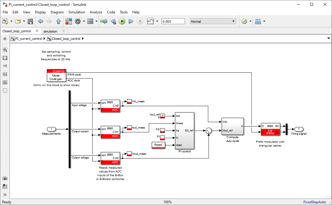
Control software

The following files contain the implementation of a current control algorithm for a buck converter in both Simulink and PLECS environments using the ACG SDK.

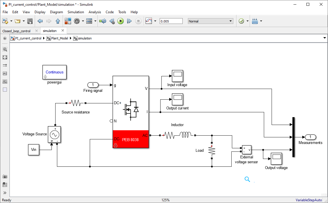
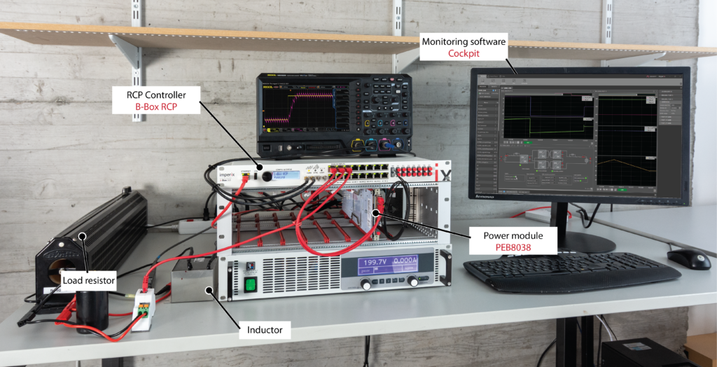
Experimental setup

Detailed step-by-step instructions for building this setup are given in PN119. The converter contains the following main components:

• One B-Box RCP controller with ACG SDK software
• 1x PEB8038 half-bridge module (rated for 800V 38A)
• 1x 2.2mH 32A inductor
• 1x 8Ohms load resistor

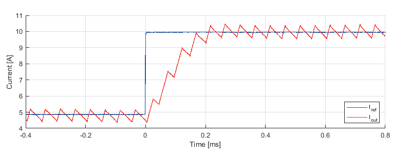
Tracking performance

The graph below shows the step response of the current control to a reference change from 5 to 10 A. The closed-loop control algorithm clearly acts as intended and follows the reference.