HIL simulation using a B-Board PRO

This technical note introduces the basic principles of HIL simulation and provides practical considerations for the implementation of a controller-HIL setup using the imperix B‑Board PRO. In the developed example, Plexim’s RT Box is used as the simulator executing the plant model in real time.

Introduction to HIL simulation

Hardware-in-the-loop (HIL) simulation is generally defined as a validation technique where a real physical controller interacts with a simulated plant instead of the actual physical plant. The controller is therefore the hardware inside the (control) loop involving an emulated system, the latter being often implemented using dedicated real-time simulation equipment. A HIL test bench typically consists of:

• Real-time simulator: executes the plant model, often with a fixed time step.
• Controller: runs the control algorithm on the real control hardware.
• I/O interface layer: connects the controller with the simulator.

This configuration is often referred to as controller-HIL (or C-HIL), because the controller is the device under test (DUT) inside the loop. Other configurations of “hardware inside the loop” are also possible, for instance involving an emulated controller connected to a real plant (opposite configuration), although this is usually not designated as a HIL setup. In the same line of ideas, the configurations that involve real power exchanges are rather designated as Power HIL (or PHIL) scenarios, so that they are clearly distinguished from those that only exchange signals or information. In this case, a power amplifier (or equivalent) is required between the simulator and the DUT.

HIL and PHIL simulation are widely used in domains such as power electronics, automotive, aerospace, microgrids, and power systems. Their typical benefits are to help accelerate development and improve safety, notably by shifting risky or hard-to-reproduce scenarios into a secure, controlled environment.

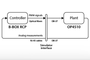
In a typical C-HIL configuration, illustrated in Fig. 1, the simulator computes the plant response in real-time and emulates the corresponding physical sensor signals (such as voltages and currents) that the controller would otherwise receive in an actual deployment. These signals are exchanged through a physical I/O interface, creating a closed loop. On the other side of the interface, the controller sees the simulator through the same analog and digital interfaces, “believing” that it is connected to the real system.

Offline vs. real-time simulation

In order to compute the plant response in real time, the simulator must be able to solve the corresponding differential equations within a pre-determined latency. For this reason, the model must be compatible and optimized for fixed-step execution. Iterative solvers are typically avoided. Additionally, the model fidelity must be chosen as a trade-off, so that the simulator can reliably finish computation before the next time step. Over-runs are generally considered as a real-time violation.

Due to the above constraints, discrepancies between offline and real-time simulation can often happen. Some typical situations are mentioned below:

• Offline simulation might be using a solver type and configuration (i.e., variable-step or fixed-step) that resolves switching and fast dynamics differently than the real-time solver being used by the simulator.
• Real-time simulation forces a compromise between time step and model complexity, which can result in changes in high-frequency behavior and transient performance.
• The controller generates PWM edges almost continuously in time, but the real-time simulator sees them through a discrete-time capture interface. If edges don’t align exactly with the real-time step, edge timing quantization happens, which significantly distorts the duty-cycle estimation, especially for high switching frequencies. All HIL vendors implement techniques to minimize this effect, with different pros and cons.

Imperix interfaces for HIL simulation hardware

Imperix offers different rapid control prototyping (RCP) controllers, power modules and sensors, enabling users to perform experimental validation of control algorithms. For HIL simulation scenarios, the B-Board PRO (e.g. mounted on its Eval-Board) can easily be interfaced with third-party HIL simulators using appropriate cables, such as a DB-37 pigtail cable. Conversely, for the family of B-Box controllers, imperix provides dedicated simulator interfaces that serve as a physical bridge between the controller and the simulator. These interfaces ensure electrical and signal-level compatibility for both analog and digital signals:

• Analog outputs of the simulator are converted to RJ45 connectivity for the B-Box controllers.
• Optical PWM signals from B-Box controllers are converted to electrical signals for the simulator.

Imperix currently provides the following simulator interfaces that allow the connection to the respective HIL simulation platforms:

• OPAL-RT Simulator Interface, refer to TN180 for further details on simulation with OPAL-RT simulators.
• Typhoon HIL Simulator Interface
• Plexim RT Box Simulator Interface
• Speedgoat Simulator Interface

Benefits and limitations of HIL simulation

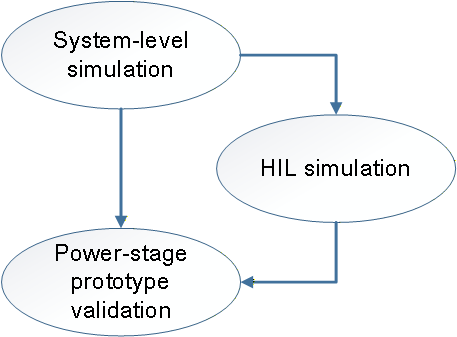
In a typical development process, HIL simulation can serve as the bridge between simulation and hardware testing, as illustrated in Fig. 2. It is an optional step that can help validate controller algorithms early in the development process, typically when a hardware prototype is not yet available or when offline simulations are inconveniently long to execute.

HIL simulation is particularly useful when testing involves difficult or destructive scenarios that are unsafe, costly, or impractical to reproduce on physical prototypes (e.g., fault injection, AC grid disturbances, over-current events, etc). More generally, HIL simulation also brings increased realism compared to offline simulation by:

• Forcing the incorporation of real-world challenges such as measurement noise, quantization phenomena, discrete control execution, hardware-specific limitations (e.g. memory usage, stack overflows), etc. inside the simulation.
• Offering support for testing random interactions such as perturbations, communication exchanges, etc.

On the other hand, HIL simulation also possesses some inherent limitations, such as:

• Dynamics close to the discretization step size are difficult to model or cannot be modeled with sufficient accuracy. While this is obvious for very fast phenomena (e.g., semiconductor ringing), this often also applies to medium-frequency dynamics (e.g. DAB or LLC waveforms), at least without highly dedicated FPGA-based solvers (which generally offer only limited user flexibility or observability).
• Evaluating system efficiency is generally not feasible, because any efficiency results merely reflect the assumptions of the underlying models (rather than validating actual physical hardware losses).
• Phenomena related to the common-mode behavior of the system are generally ignored (due to the associated computational burden, incompatible with real-time execution), imposing limited visibility on the possible issues associated to filters, circulating and leakage currents, etc.
• More generally, any aspect that is not anticipated and, therefore, included in the simulation model cannot be faced or tested. This prevents HIL simulation from being able to expose unforeseen challenges or problems.

In light of the above, the value of HIL simulation lies not so much in improving the plant model fidelity, but rather in offering what offline simulation lacks, i.e.:

• Testing opportunity for the real control hardware along with the embedded software or firmware.
• Offering support for faster simulations with faster iteration cycles, as they run in real-time on dedicated hardware.

In practice, HIL simulation is generally cost-effective when it prevents expensive prototype iterations by catching integration- and control-related issues early, while prototyping is attractive and necessary when the dominant risks are related to the power stage, or involve efficiency- and EMC-related concerns.

C-HIL simulation example

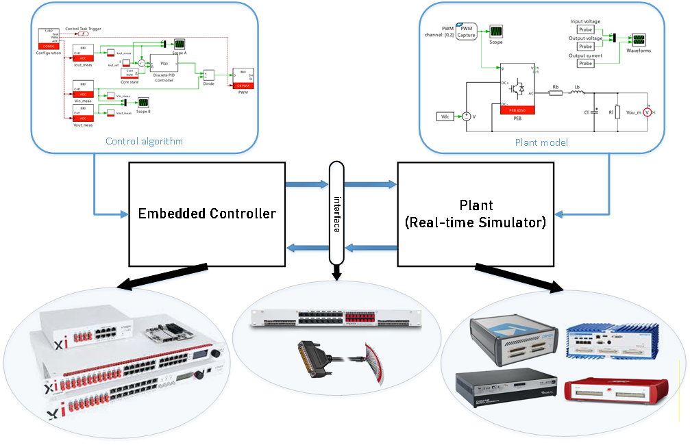
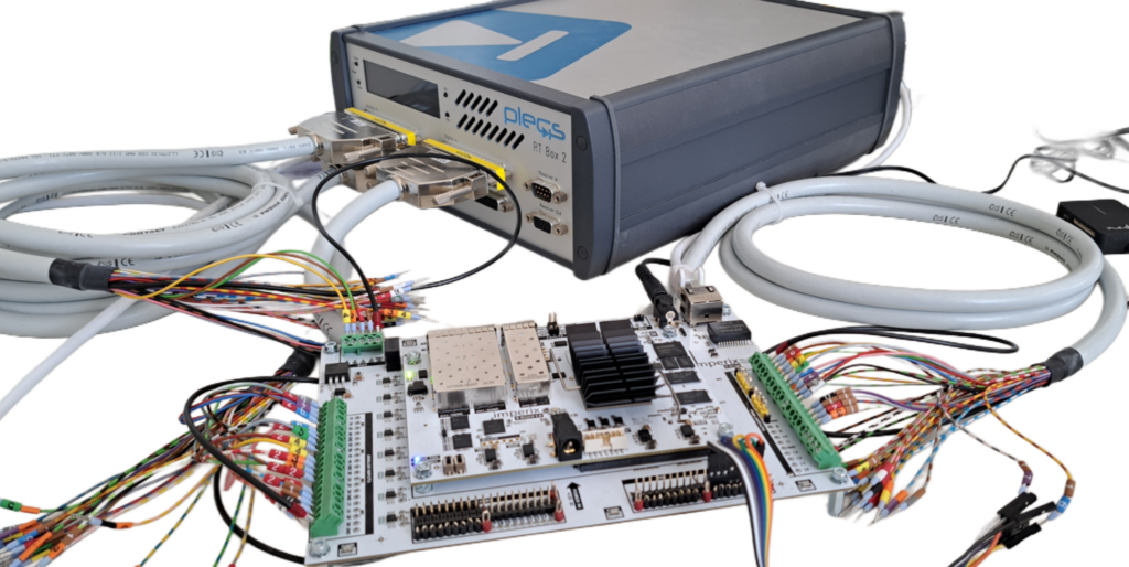
This example uses the imperix B-Board PRO and Plexim’s RT Box 2. The real-time simulation of a DC-DC buck converter is used to demonstrate the workflow using PLECS. TN100 outlines the implemented output voltage control and is used as a reference. The simulation model is built using the imperix Power library.

In this example, a single PLECS model is used to generate C++ code for both the control side and the plant side, which are subsequently deployed to the  B-Board PRO and Plexim RT Box, respectively. Specific settings may differ for other real-time simulators, but the underlying concepts remain the same. The following articles address the corresponding steps and are recommended for further reading:

• PN134 for getting started with imperix ACG SDK
• PN137 for understanding simulation essentials with PLECS
• PN151 for other PLECS examples with different plants available for download
• AN006 for a similar implementation of HIL simulation using the B-Box RCP 3.0 and Plexim’s RT Box 2

Downloads

A PLECS model containing the closed-loop output current control of the DC-DC buck converter is provided. The imperix power library requires ACG SDK 2024.2 or a later version.

Experimental setup

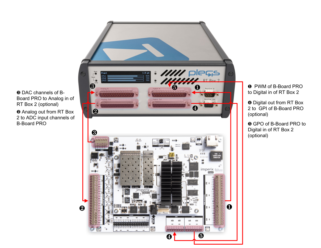
The experimental setup is shown in the Fig. 3. An exploded DB-37 cable is used to connect the B-Board PRO development kit with the front side of the RT Box. While in this note, this specific setup is featured, other imperix controllers can also be utilized in conjunction with their corresponding simulator interfaces.

Hardware and software requirements

The following list includes imperix products, plus additional components required for this example:

• Imperix products
  • 1x B-Board PRO development kit
  • Imperix Control development tools for Simulink and PLECS (ACG SDK) that includes Cockpit
• Additional software
  • PLECS standalone with PLECS coder
• Additional hardware
  • Plexim RT Box (can be any variant)
  • 2x exploded DB-37 cable
  • 1x DB-37 gender changer
  • 12V DC adapter for powering the B-Board PRO

Setting up HIL simulation

The setup of HIL simulation involves several steps. A similar procedure can be followed for setting up a HIL simulation with any other control implementation or plant model.

Model implementation

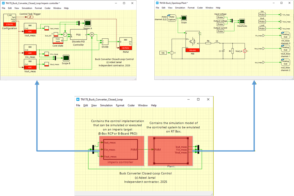
A buck converter example is built in PLECS using the default template file provided by imperix. The controller and the plant are modelled in seperate subsystem as shown in Fig. 4.

PLECS model preparation and settings

Effective data exchange between the RT Box and the B-Board PRO relies on several key blocks from the PLECS RT Box library (italicized below) and the imperix library (in bold red below). Below are the critical considerations for their implementation:

• PWM capture blocks must be used for receiving the PWM signals (as opposed to regular digital input blocks) so that sub-cycle averaging is possible. The offline behavior in the PWM capture block should be selected as sub-cycle average to properly mimic the real-time behavior. Nanostep is only compatible with Nanostep-compatible models from the PLECS library.
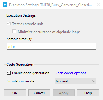
• As the model will be deployed in the RT Box, the subsystem containing the plant side must be enabled for code generation. For that, right-click on the plant subsystem and select subsystem–> execution. Then check “enable code generation”, as shown in Fig. 9.
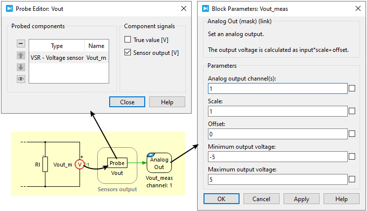
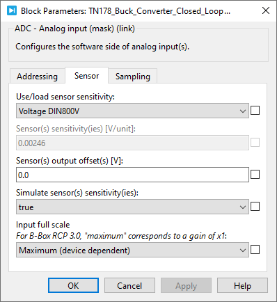
• Analog output blocks on the RT Box should be used to provide the plant measurements to the imperix ADC blocks. To reflect the physical scaling of the real-world hardware, it is recommended to scale these signals according to the actual sensor sensitivity by probing its “Sensor output [V]” signal (see Fig. 5). On the controller side, the ADC must be configured with the corresponding sensor parameters (Fig. 6) to ensure the scaling matches. This configuration can be validated during offline simulation by enabling the “Simulate sensor sensitivity” option within the ADC block settings.
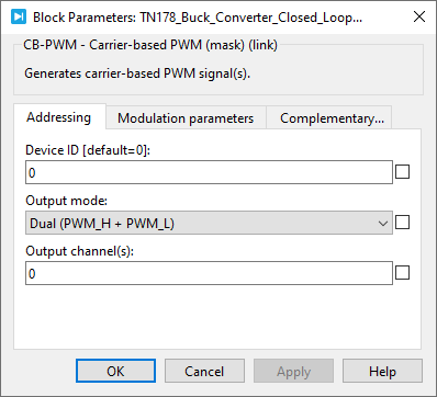
• The recommended settings for the CB-PWM block are shown in Fig. 7. As both PWM signals are generated and transmitted to the simulator, reverse conduction is implemented in the lower MOSFET.

The following are some optional interfaces included for the sake of completeness. They can be used, for example, when control logic or relaying is required:

• Digital In can be used for general-purpose output signals (GPO) coming from the B-Board PRO.
• General-purpose input signals (GPI) from the B-Board can be connected to the Digital Out of the RT Box.
• DAC channels can be used to output analog signals from the B-Board PRO. The imperix DAC block and the corresponding Analog In of the RT Box library can be used.

Wiring of the B-Board and RT Box

The system is wired as follows, which is illustrated in Fig. 9:

• The PWM outputs of the B-Board PRO are wired to the RT Box digital inputs. An exploded DB-37 cable can be used to wire them together as shown in Fig. 3.
• The analog outputs of the RT Box are wired to the analog inputs of the B-Board PRO.

Deployment of the plant model

The step-by-step procedure to compile and load the plant model on the RT Box is as follows:

• If not already, code generation must be enabled for the subsystem containing the plant side. Right-click on the plant subsystem and select subsystem–> execution. Then check “enable code generation”, as shown in Fig. 8.
• In the PLECS environment, go to Coder→ Coder options. Select “plant” in the left area (under the model file name).
• The “General” tab can keep the default settings.
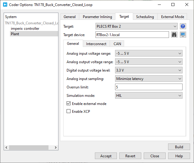
• In the “Target” tab:
  • Select the RT Box variant being used. In this example, PLECS RT Box 2 is selected.
  • Select the analog output voltage range to “-5V … 5V” as B-Board PRO’s input voltage range is ±5V.
  • Select HIL for the simulation mode. All the settings for the “Target” tab are shown in Fig. 10.
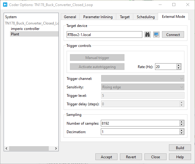
• In the “External mode” tab of the coder options menu:
  • Select the target device by entering the hostname or IP address. Other settings are shown in Fig. 11.
  • Click “Build” to generate and upload the code directly to the RT Box.
  • When everything is rightly done, a blue LED next to “Running” on the front interface of RT Box 1 will light up. For other RT Box variants (e.g., RT Box 2 used here), the LCD will display the name of the subsystem being simulated in addition to the current CPU cores’ processing time.

Deployment of the control implementation

The following steps outline how to compile and load the control algorithms onto the B-Board PRO. More information on how to program and operate imperix controllers is provided in PN138:

• The subsystem containing the control side must also be enabled for code generation. Right-click on the controller subsystem and select subsystem–> execution. Then check “enable code generation”, as shown in Fig. 8.
• Open Coder → Coder Options, then choose “imperix controller” from the panel on the left (under the model name).
• The “General” tab can keep the default settings.
• Go to the “Target” tab and select “Imperix Gen 3 Controller”. In case B-Box 4 is used, then “Imperix Gen 4 Controller” should be selected.
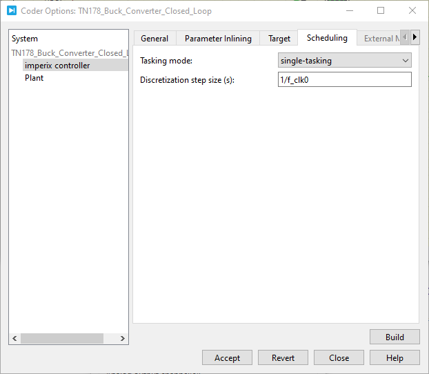
• Go to the ” Scheduling” tab:
  • Select “single-tasking” under Tasking mode
  • The discretization step size must be set equal to the control time period, as shown in Fig. 12.
• Click “Build”. Imperix Cockpit should open up automatically.

Testing and validation

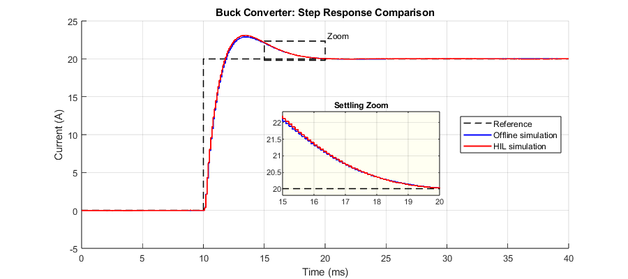
The results of offline simulation in PLECS as well as HIL simulation are captured and presented in Fig. 13. In this example, the switching frequency of the buck converter is set to 10kHz. With a fixed discrete time step of 2µs, the RT Box executes the model at 500 kHz (f_s), which is sufficient to resolve dynamics around the buck’s switching frequency. However, it cannot represent any dynamics above the Nyquist limit of 250 kHz. In practice, the usable frequency range is typically much lower, in the order of 50 kHz (≈ f_s/10). As a result, phenomena faster than this are not captured realistically.

The following can be observed:

• By keeping the electrical and control parameters identical in both offline and HIL simulations, and by accurately modeling delays in the offline model, both results show an essentially identical response to a step change in the output current reference. The offline and real-time HIL waveforms align closely, as also seen in the zoomed settling-time view.
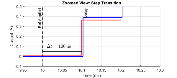
• The reference step is applied at 10ms and, as expected, the controller response is visible at the next interrupt execution (i.e., after 100µs). This behavior is consistent for both offline and HIL simulations, as shown in Fig. 14. Sampling, actuation, and response timing are all observed to be coherent.

If the model is complex and overruns occur during real-time deployment, iterative adjustments to plant fidelity and time steps may be necessary to balance real-time constraints with test objectives.

Getting-started recommendations

Conclusion

The workflow utilizing the imperix B-Board PRO and Plexim’s RT Box demonstrates seamless compatibility between the controller and the real-time simulator. Comparative results reveal equivalent delays and dynamic responses across both offline and HIL simulation environments, confirming the correct interaction between the devices.

These findings suggest that HIL simulation can be an attractive alternative to offline simulation, offering increased realism, when the perspective is set on the control hardware testing. In such a case, the ability to conduct testing early along the development cycle provides benefits that outweigh the limited accuracy of the model (such as a restricted frequency range or disregarded common-mode behavior). That said, more generally, HIL shall rather be seen as a complement than a replacement to offline simulation. Notably, HIL should not be considered blindly as a method for achieving higher modelling accuracy, which it isn’t.

When opposed to experimental prototyping, HIL simulation is an excellent framework for executing tests that are either hazardous or difficult to replicate in a laboratory setting. It is also often faster and less cumbersome than physical testing. However, thermal and EMI-related phenomena typically remain outside the scope of current HIL capabilities. Additionally, the cost-effectiveness of HIL versus full-scale prototyping remains a subject for further debate.

To go further from here…

The next step could be to implement the buck converter physically and test the controller’s performance. Refer to PN119 to understand how to build a buck converter from scratch using imperix half-bridge modules and sensors. The following resources can also be helpful:

• TN100: Step-down buck converter
• TN180: C-HIL simulation scenario with OPAL-RT simulators
• TN122: Interleaved buck converter current control
• TN102: Buck-boost converter
• PN151: Basic examples for ACG SDK on PLECS