Parametric system identification using the imperix Sys. Id. toolbox

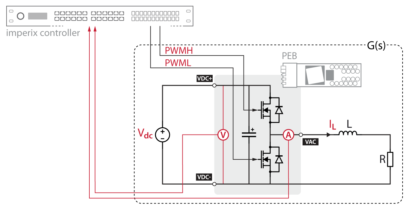
This note illustrates a system identification example that derives a parametric model using the imperix System Identification toolbox. It presents a step-by-step procedure, starting by preparing the Simulink/PLECS model, performing the frequency response measurement, and finally deriving the parameters. The example considers a buck converter with an inductor and a resistor connected at its output, and the goal is to identify their values.

Hardware requirements

The following list describes the elements used to build the buck converter:

• A phase leg module (PEB-800-40, PEB8038, PEB8024, or PEB4050);
• A programmable controller (B-Box 4, B-Box 3, or B-Box 3 Micro);
• Control development tools for Simulink/PLECS (ACG SDK), with a valid license;
• A DC power supply;
• An inductor and a resistor;

Identification procedure

The procedure to identify the system parameters divides into two main steps:

1. Identify the frequency response from the duty cycle to the inductor current;
2. Derive its analytical expression and parameterize it using the identified response.

Since the system is known, it’s possible to make assumptions about the roles of the various components using the laws of physics. In this case, the RL series dynamics will dominate the frequency response mentioned in step 1. After finding an appropriate analytical expression, parameterizing it yields the inductance and resistance values by finding the numerical values that fit the measured frequency response.

The imperix System Identification toolbox implements the Empirical Transfer Function Estimation (ETFE) technique to estimate the frequency response between two signals. This requires deciding where to perturb the system and which two signals to record to compute the frequency response from one to the other. For more details regarding the ETFE implementation, see the Sys. Id. Injector block documentation.

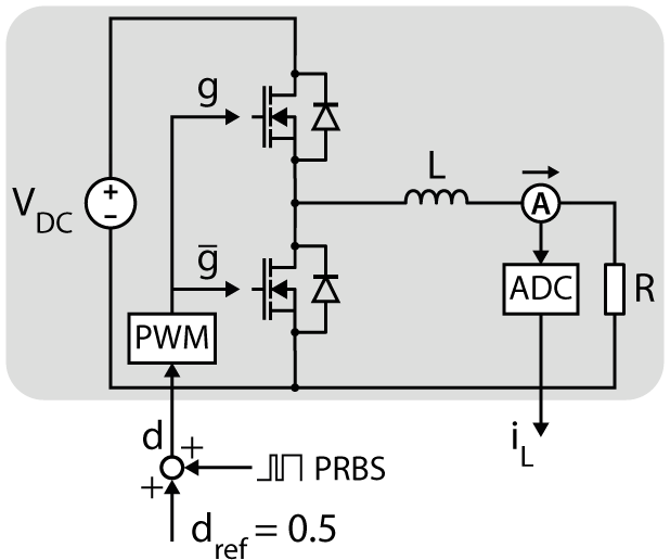
As the frequency response of interest is from the duty cycle to the inductor current, it is reasonable to inject the perturbation on the duty cycle and to measure the perturbed duty cycle signal d and inductor current i_L. The following schematic depicts the identification setup, where the grey area shows the identification target.

Simulink and PLECS models

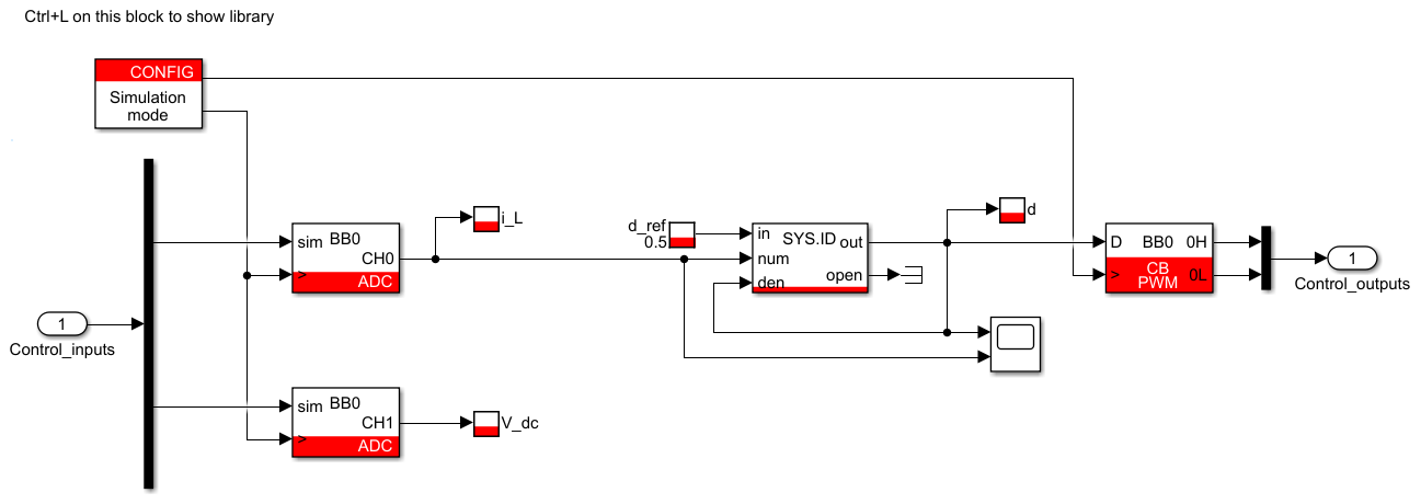
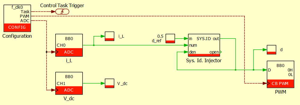
The following Simulink and PLECS models implement the setup shown above. The perturbation signal is injected using the Sys. Id. injector block, connected between the duty-cycle reference and the PWM modulator input, matching the configuration above. The probe blocks are used to acquire in Cockpit the duty cycle d and inductor current i_L.

Identification in Cockpit

To build and deploy the models to an imperix controller by pressing Ctrl + B in Simulink or Ctrl + Alt + B in PLECS. More information is available in PN138. After building the model, Cockpit will open automatically. It will also automatically detect the Cockpit project file (.ixproj) provided with the models. This pre-configures the project workspace by adding a Scope module and a System Identification module, and adds the i_L and d variables to the Scope, which are needed by the Sys. Id. module.

Identification procedure

Once Cockpit is open, the following steps detail how to perform the identification process:

1. Turn on the DC voltage source and make sure the variable V_dc settles around the expected value. In this case, it’s set to 200 V. If not, check the sensor’s sensitivity and whether it is connected to the correct channel. The PWM enable switch should be off, so i_L should be zero.
2. The tunable reference signals should bring the system to the desired operating point. In this case, as the duty cycle ranges in [0,1], d_ref = 0.5 provides equal headroom in both directions for the PRBS signal.
3. The options on the right panel (under the Sys. Id. section) configure the injection parameters:
   • Since the system has no control loop, setting Injection mode to open-loop or closed-loop makes no difference.
   • The perturbation amplitude should yield a good signal-to-noise ratio without introducing harmonics that would reduce estimation accuracy (i.e., avoid non-linear operation). In this case, 0.1 is a good starting point.
   • The advanced parameters are left at the default value in this case. The PN306 provides more information on these.
   • The numerator and denominator signals should be chosen according to the frequency response of interest; in this case, from the duty cycle to the inductor current. Then, d is the denominator and i_L is the numerator.
4. Enable the PWM and ensure the resulting current is constant.
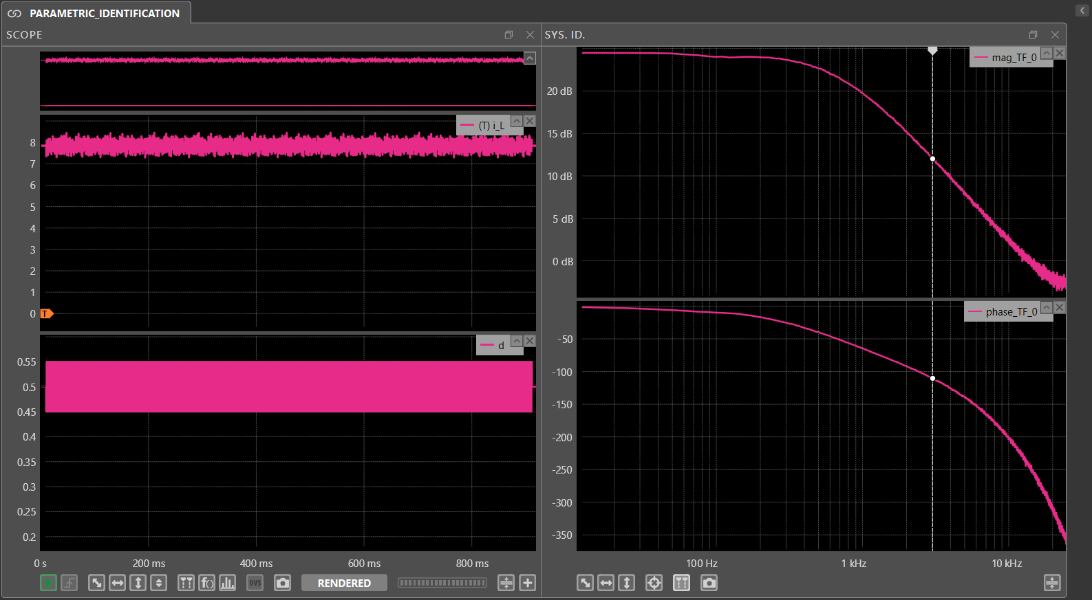
5. Press the start injection button, wait for the injection to end, and the Bode plot of the identified transfer function will appear. The picture below illustrates the obtained result.
6. The waveform can be exported for later processing with the right-click menu (.csv or .mat). Alternatively, snapshots can help in comparing multiple acquisitions.

Parametrization of the transfer function

The previous section yielded the frequency response from the duty cycle to the inductor current, and it is possible to derive an analytical expression for it. For the buck converter under consideration, it can be a first-order system [1]:

The above transfer function neglects the delay due to PWM and sampling, as it is not needed to derive the inductance and resistance values. The expression can be parametrized using the low-frequency and high-frequency regions of the identified frequency response. For small and large values of $\omega$:

To compute R, the appropriate frequency value is the lowest one available. Choosing $\omega$ to derive $L$ is a more delicate task: due to unmodeled parasitic elements, the above approximation holds only up to a certain frequency, that is, where the slope of the magnitude Bode plot is −20 dB/dec. For this system, 3 kHz falls almost in the middle of that region. The user can easily read the required values using the cursors, as described in the Sys. Id. module documentation:

• $\omega\approx2\pi\cdot12.2\,\mathrm{Hz}$ yields $|G(j\omega)| \approx 24.49\,\mathrm{dB}\approx16.77$, which yields $R\approx11.9\,\Omega$;
• $\omega\approx2\pi\cdot3\,\mathrm{kHz}$ yields $|G(j\omega)| \approx 12.05\,\mathrm{dB}\approx4$, which yields $L\approx2.65\,\mathrm{mH}$.

Simulation validation

This section compares the results of two different simulations, one with nominal L and R values (2.2 mH and 11.5 Ω) and one with identified ones, with the experimental data previously obtained. To run the identification in simulation, users should also enable the block for simulation, as discussed in SD041. The same settings can be used as in the experimental identification procedure. These Simulink and PLECS models are already configured to identify the system in simulation, and the following plot reports the obtained data:

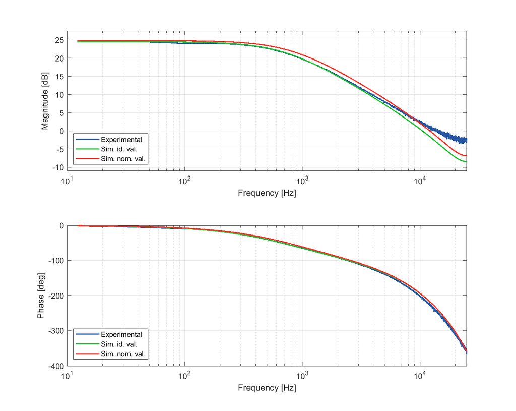
The identified values better represent the system than the nominal values, at least within the frequency range typically considered for controller design [1].

Visualizing simulation data in PLECS

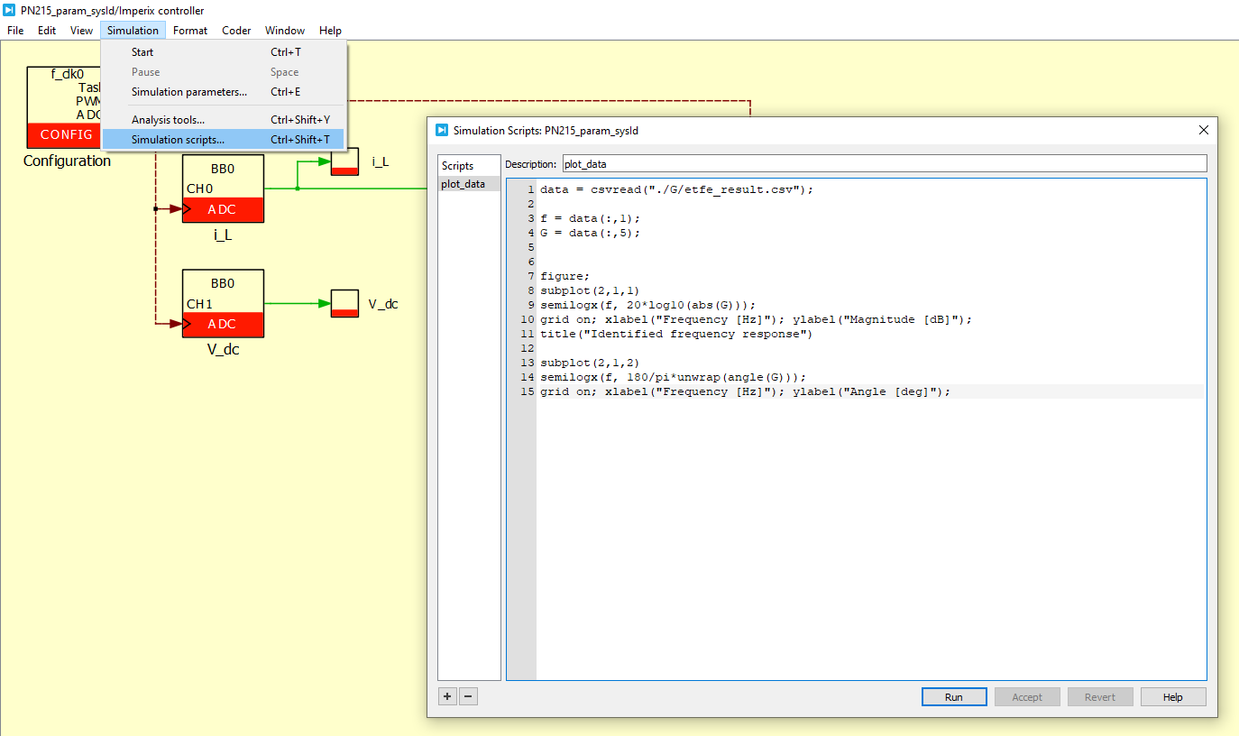
Simulink automatically plots the system’s frequency response at the end of the simulation. In PLECS, the injector block saves data to two .csv files in a folder named after the specified injector. To reduce the friction of writing custom code to plot the data, the PLECS model provides a GNU Octave script. Users can manually run it at the end of the simulation as follows:

Conclusions

The note demonstrated a procedure to identify the frequency response of the duty cycle to inductor current transfer function for a buck converter. Then, it presented a simple way to parameterize it as a first-order system, yielding inductance and resistance values that better fit the actual system behavior than the nominal values in the typical frequency range of interest (20 to 10 times below the switching frequency). A higher-order simulation model would also allow characterization of parasitic elements, improving matching in the high-frequency range. This requires determining which elements to use and how to connect them.

Further reading

It is also possible to use the system identification data to design or validate a controller in the frequency domain, as described in PN216. This note demonstrates how to derive the parameters necessary for the tuning procedure from the Bode plot, as well as how to fine-tune the controller directly in the experimental setup.

References

[1] R. W. Erickson, D. Maksimović, Fundamentals of Power Electronics, Springer, 2020