
Table of Contents
This article describes how to use the Cockpit FFT/THD module to interact with the user code running on imperix controllers. The page provides a detailed explanation of all of the module’s features.
For users seeking getting-started assistance with Cockpit itself, a separate article is available in PN300.
FFT/THD module basics
The FFT/THD module allows the user to examine variables Scope module data in the frequency domain. User variable and oversampled variable data acquired by the Scope, as well as math variable data calculated by the Scope, can be viewed in this way.
To transfer variables already in the Scope module to the FFT/THD module, right click on a variable or plot area and select the ‘Plot in FFT/THD module’ option in the context menu that appears. A variable doesn’t have to be displayed in the Scope to be acquired and displayed by the FFT/THD module.
FFT/THD module interface
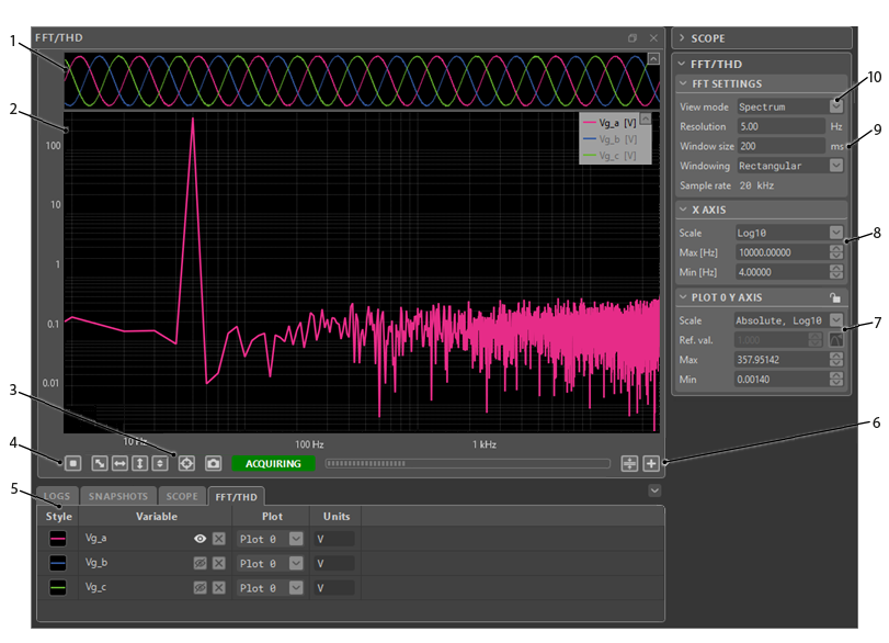
Calculating and displaying spectral content
In the FFT/THD module, the signal spectra are calculated using a variation of the Fast Fourier Transform (FFT) algorithm. Similarly to math variables in the Scope module, the calculations are performed on the PC side, after the acquisition of a scope window.
Spectrum mode
The Spectrum mode gives the best visual overview of the spectral content of the scoped signals. Since the widest window results in the highest frequency resolution, the default FFT window in this mode is the same as the acquisition window.
Technical details
The displayed frequency domain signal is the magnitude of the one-sided spectrum of the scoped variable, with the frequency range \(f \in [0, \frac{f_s}{2}]\). The Scope sampling rate, \(f_s\), corresponds to the control task frequency defined in the user code. The frequency resolution of the resulting spectra depends on the window in time over which the Fourier transform is performed and can be adjusted in the FFT Settings menu in the right bar.
Harmonics mode
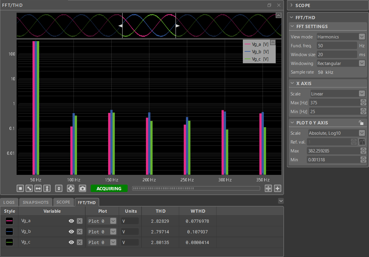
In the Harmonics mode the spectral content is calculated with the same method as in the Spectrum mode, but is plotted in a way that makes it easier to visualize and compare the individual harmonics between of different signals. In addition to this, the Total Harmonic Distortion (THD) and Weighted THD (WTHD) metrics are calculated and updated in the bottom bar menu for the variables that are currently displayed in the plot. As is typical for the Power Electronics domain, the default FFT window is such that the frequency resolution is 50 Hz.
Technical details
THD is defined as ratio of the root-mean-square of the harmonic content and the fundamental frequency, typically taken to be 50 or 60 Hz. In the FFT/THD module, THD is calculated according to the following formula:
\(\text{THD}=\frac{1}{V_1}\sqrt{\overset{\infty}{\underset{i=2,3,\dots}{\sum}}V_i^2}\),
where \(V_1\) is the amplitude of the harmonic at the fundamental frequency and \(V_i, i\in\{2,3,\dots\}\) are the amplitudes of the harmonics at the \(i\)-th multiple of the fundamental frequency.
WTHD is calculated in a similar manner, except the harmonics are weighted to be inversely proportional to their order:
\(\text{WTHD}=\frac{1}{V_1}\sqrt{\overset{\infty}{\underset{i=2,3,\dots}{\sum}}(\frac{V_i}{i})^2}\)
Interacting with FFT/THD module graphs and plots
The FFT/THD module consists of one or more plot areas that display graphs based on variables defined by the user code. This section lists out the tips and tricks for manipulating plot variables and plot areas in the module.
Managing plot variables
To add a variable to a plot, select it in the USER VARIABLE, ANALOG INPUTS or DIGITAL I/O section in the project pane, drag and drop it over the plot. To add multiple variables to a plot, keep the Ctrl key pressed and click on the desired variables to select them. Alternatively, click on the first variable to select it, keep the Shift key pressed, and click on the last variable to select. Variables selected like this can then be dragged and dropped into a plot all at once.
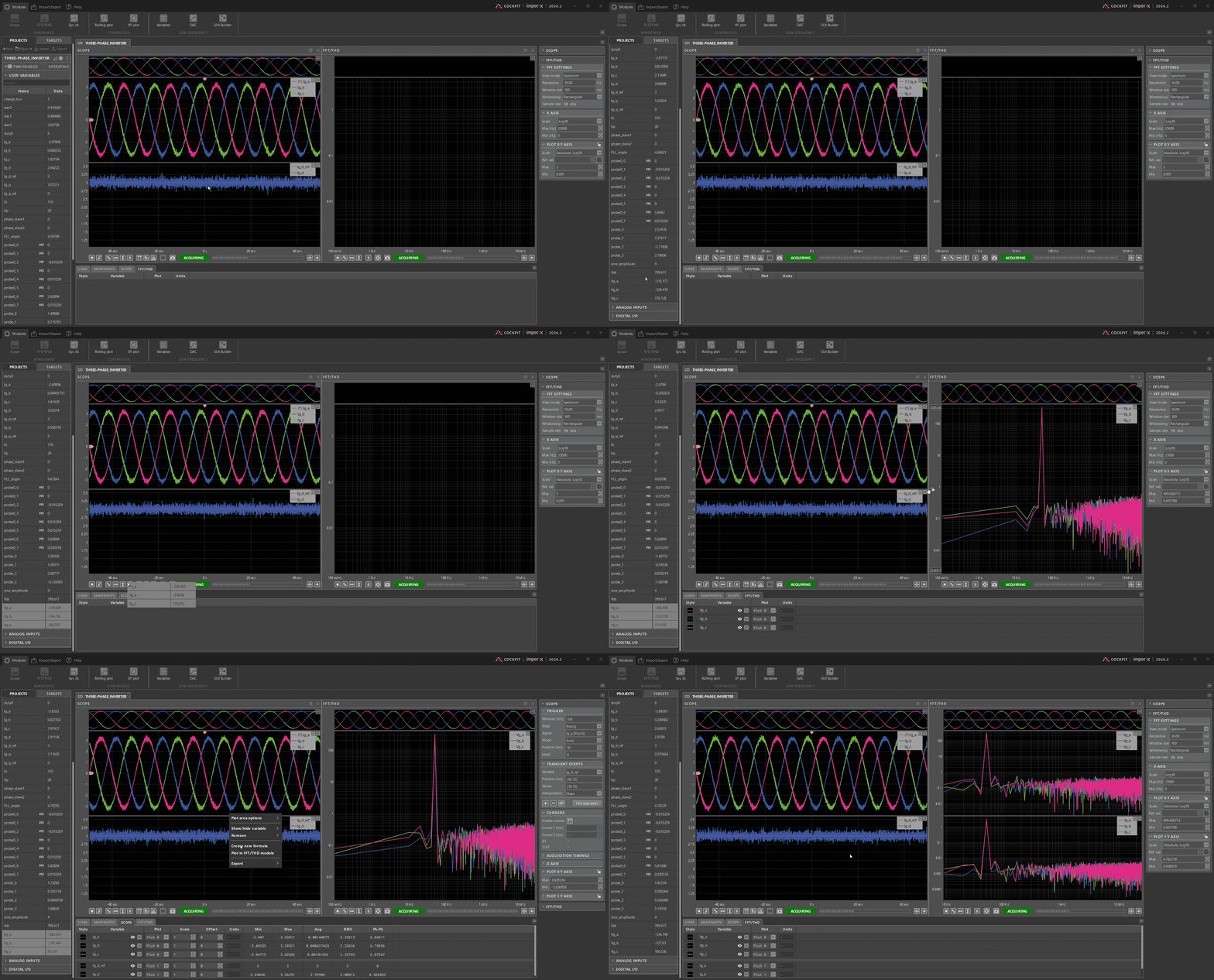
Added variables will show up as rows in a table in the bottom bar tab corresponding to the module. Here, variables can be removed, their style and visibility and plotting order can be managed and they can be moved from plot to plot. In the Harmonics mode, the THD and WTHD metrics are shown as well.
All of these actions can also be accessed from context menus by right-clicking on a plotted variable or on the empty space in the plots.
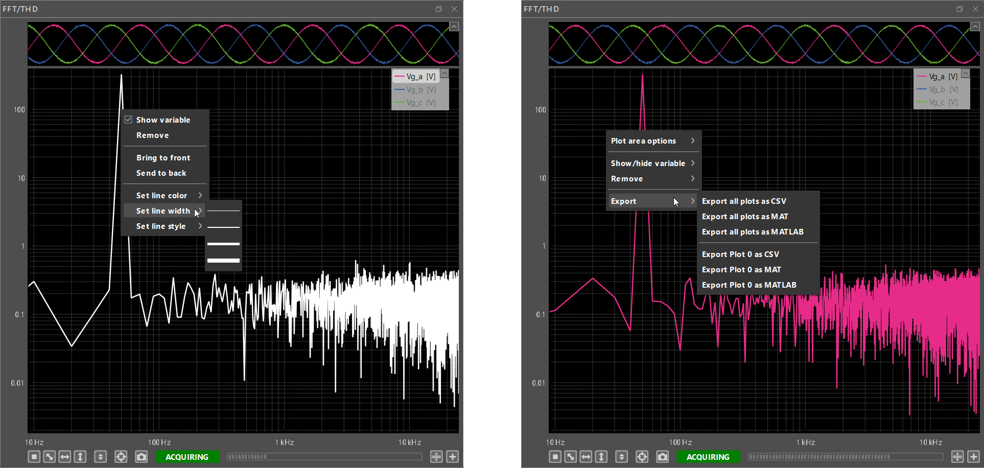
Managing plot areas
New plot areas can be added by clicking on the + button in the bottom right of the module. The total module height can be freely distributed between the plots. To resize plot heights click on the border between the plot areas and drag.
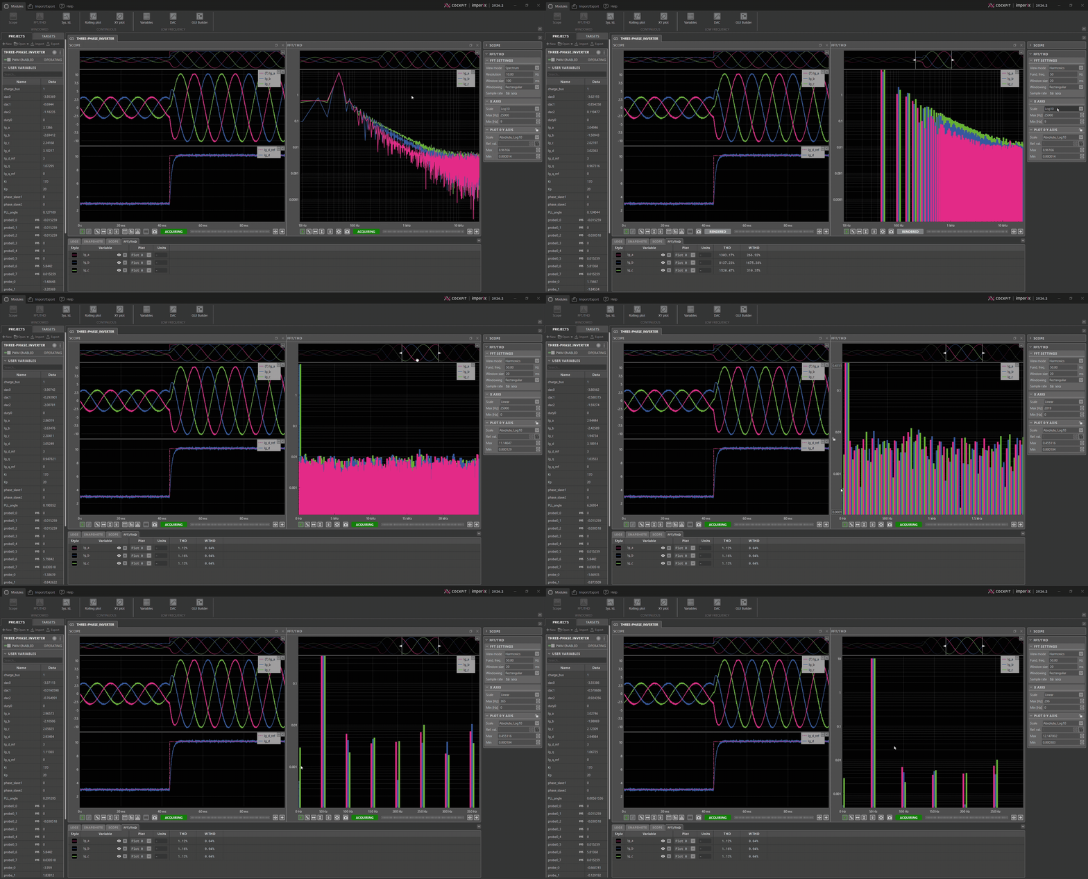
- To zoom in and out along the horizontal axis, place the mouse cursor over the area of interest. Then, use the mouse wheel to zoom in or out around the location of the mouse cursor.
- To zoom in and out along the vertical axis, place the mouse cursor over the area of interest. Then press the Ctrl key and use the mouse wheel to zoom in or out around the location of the mouse cursor.
- To zoom on a specific area, click and drag to draw a blue rectangle over the zoom area.
- To achieve a horizontal auto-scale, right-click and drag horizontally. A light grey horizontal strip will appear. Release the mouse button to perform the horizontal auto-scale.
- To achieve a vertical auto-scale, right-click and drag vertically. A light grey vertical strip will appear. Release the mouse button to perform the vertical auto-scale.
- To enter panning mode press and hold the mouse middle button or Ctrl + Left mouse button and move the mouse.
- To prevent a plot from changing the displayed range of values, hover over the y-axis and click the lock icon that shows up. The same can be done frome the y-axis pane menu in the right bar.
 By Stéphane Lovejoy • April 12, 2022 • PN300
 By Mateja Ilić • August 25, 2025 • PN301
 By Jules Perrin • February 4, 2026 • PN305