
Table of Contents
This article presents the key functions available in Cockpit’s Scope module and provides some usage examples. For users seeking general assistance with Cockpit, getting-started documentation is available in PN300.
Scope module basics
The Scope module lets users display control variables on an oscilloscope-like interface by capturing and plotting every sample of the scoped user variables. The acquisition is performed at the control task rate (i.e., the controller’s main interrupt frequency), ensuring that every sample is scoped.
When used with the B-Box 4, the Scope also supports displaying raw data coming straight from I/O peripherals, which is acquired at a significantly faster rate. Specifically, analog inputs can be observed at a 10/20 Msps refresh rate, while digital signals are captured at 250 Msps. Overall, the scope can display:
- Up to 32 user variables (CPU) for 40 seconds, or longer if fewer signals are used.
- Over 400ms with 24 ADC channels active, or longer with fewer signals.
- Up to 2 seconds when scoping all PWM channels, or longer with fewer signals.
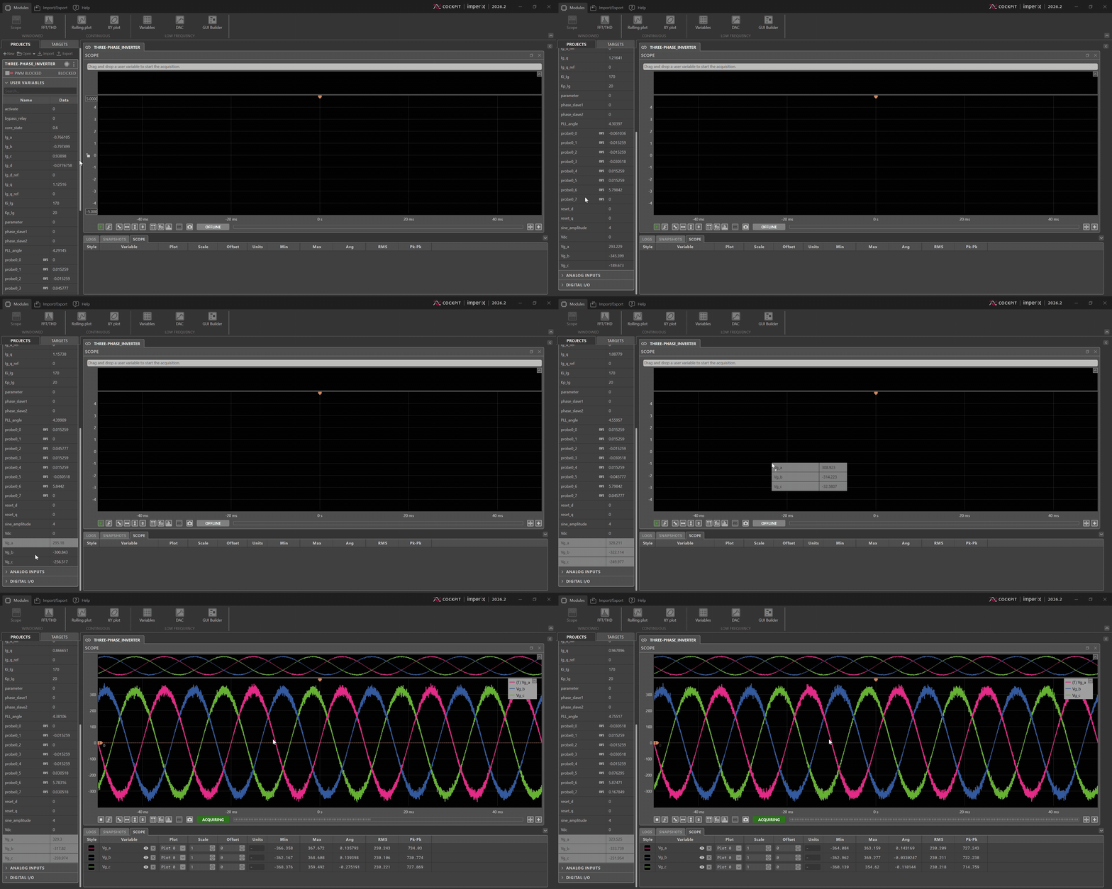
To start the acquisition, drag and drop a variable from the project pane directly to a plot of the scope module.
Scope module interface
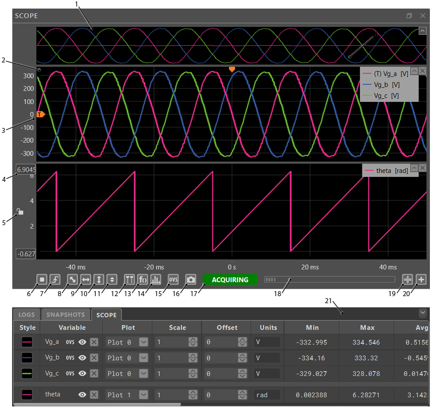
Trigger configuration
The trigger mechanism of the Scope module behaves the same way as the trigger on a regular oscilloscope. The Trigger pane, located in the right bar, allows the configuration of the scope trigger.
![Screenshot of the Scope module Trigger configuration pane in imperix Cockpit software. The panel displays several trigger settings with numbered annotations from 1 to 6, which correspond to the features detailed in the article. These point to the Window [ms] input field (1), the Edge dropdown set to Rising (2), the Signal dropdown set to Vg_a [Plot 0] (3), the Mode dropdown set to Auto (4), the Position [ms] and Level numerical input fields (5), and an enabled Ripple reject checkbox (6).](https://imperix.com/doc/wp-content/uploads/2025/08/Trigger_annotated2026.png)
Sets the duration of the acquisition window, which affects the number of points acquired and the corresponding amount of data.
Defines whether to trigger on the rising edge, the falling edge, or both edges of the chosen signal.
Selects which signal is used for triggering the Scope. Once selected, this signal is marked with a (T) in the plot legend. Only variables currently added to the Scope are present in this drop-down list.
![Screenshot of the imperix Cockpit Scope module Trigger configuration pane. The image highlights the expanded "Signal" dropdown menu, which displays various available trigger sources. The listed options include system events such as "PROTECTION TRIP" and "PWM ENABLED," user variables like "Iout_meas [Plot 0]" (which is currently highlighted/selected) and "Vin_meas [Plot 2]," as well as oversampled hardware channel signals including GPI, GPO, and PWM channels.](https://imperix.com/doc/wp-content/uploads/2025/08/trigger_signal_selection.png)
On the B-Box 4, the acquisition can also be triggered by ADC data, digital I/O channels, protection trips, or the PWM enable/disable state information. Whenever both CPU and oversampled data are available for a given measurement, the oversampled data is preferred.
Defines the trigger acquisition mode.
In Normal mode, acquisition is triggered when the signal reaches the trigger level.
In Auto mode (default), the trigger behaves as in normal mode. However, acquisition is also triggered automatically every 100 ms if no trigger event occurs in the meantime.
In Single mode, a single window is acquired when the signal reaches the defined level. After that, the acquisition is stopped.
Defines the signal level that triggers the acquisition. This can also be adjusted by manually sliding the corresponding cursor inside the plot area.
When enabled, this feature improves the stability of oversampled ADC signals by preventing undesirable triggers on ripple. See the Ripple reject section below for more details. This option is only available on the B-Box 4 with SDK 2026.2 or newer.
Oversampled signals
Oversampling refers to acquiring analog signals at a rate faster than the CPU control rate and displaying them in the Scope module. This feature is exclusive to the B-Box 4 controller. It enables the observation of analog signals across the full sensor bandwidth, supporting superior data analysis and facilitating troubleshooting.
The Scope supports two types of oversampled signals:
- ADC signals at the native acquisition rate of 20 Msps (or 10 Msps channels 12-23 are used)
- Digital I/O (PWM, GPI, GPO, FLT) signals with a resolution of 250 Msps (4ns).
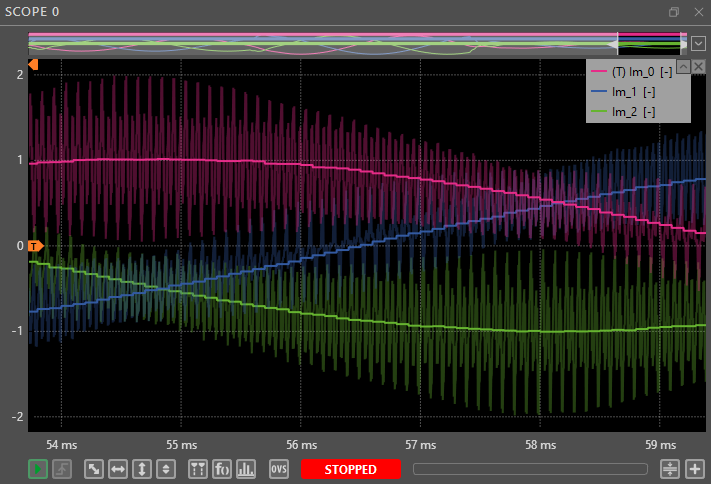
Oversampled inputs can be selected from the left bar in Cockpit. To display them, drag and drop them into the Scope like any other variable. Oversampled data is also automatically displayed for user variables that are closely connected to an ADC block in the user code. Users can then toggle oversampled data on or off by right-clicking the corresponding signal.
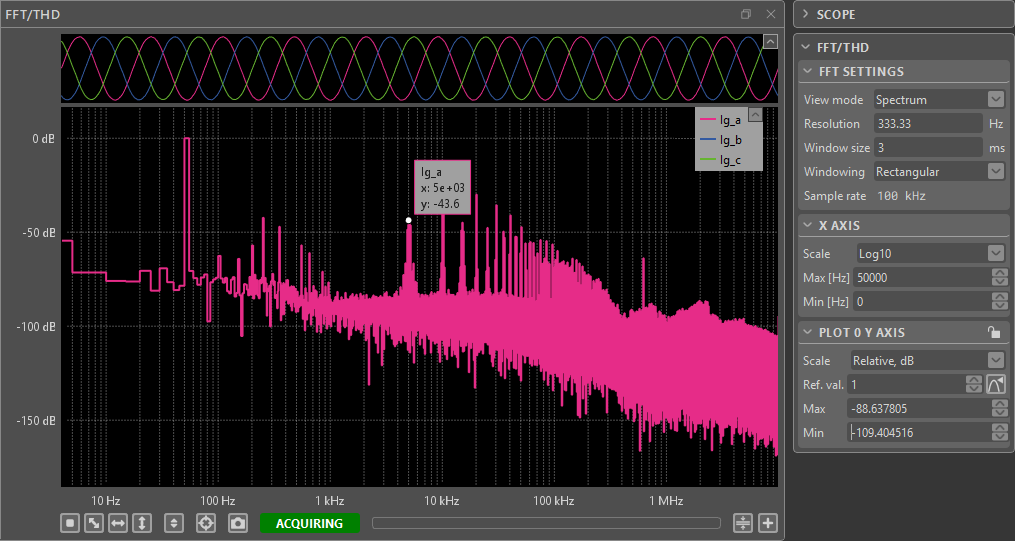
Oversampled data is also supported within the FFT/THD module, enabling analysis above the Nyquist frequency defined by the control rate. This notably permits the evaluation of switching ripple.
Ripple reject
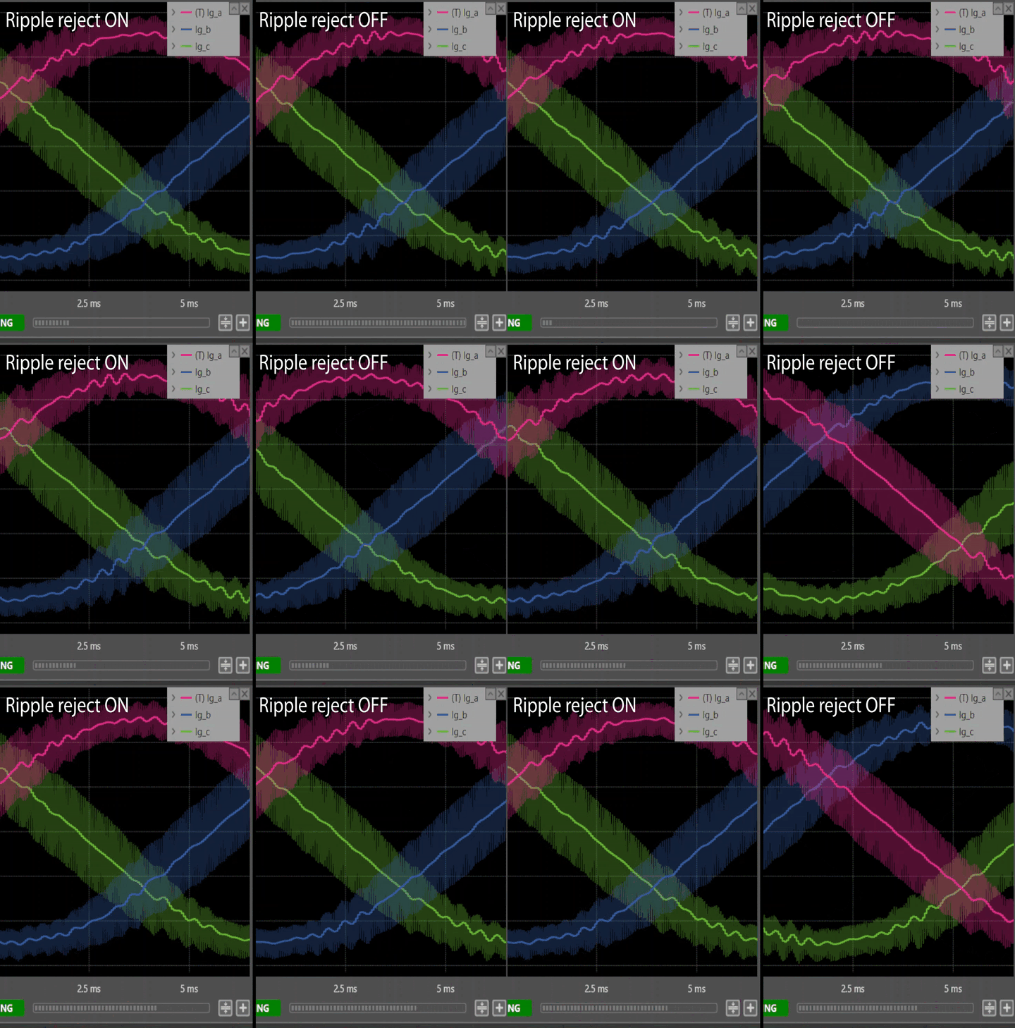
Oversampled signals often contain inherent ripple and high-frequency noise. Triggering on such signals may hence be difficult, resulting in unstable, jittery plots that are difficult to read and analyze.
To avoid false triggering and stabilize the display, the Ripple Reject function adds a trigger condition that ignores minor signal fluctuations and high-frequency ripple. The Ripple Reject mode is enabled by default, but can be disabled if needed. It is only available on the B-Box 4 with SDK 2026.2 or newer.
Transient generator
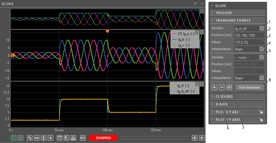
The transient generator allows users to define and impose stimuli on user variables. Both steps and ramps can be applied to any writable variable, such as those linked to a Tunable parameter block. If desired, transients can be applied to multiple variables simultaneously.
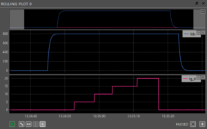
The Transient generator is typically useful for evaluating the transient response to reference steps (tracking performance) or external influences (perturbation rejection). In the example shown below, three consecutive steps are applied to Ig_d_ref, so that the current control performance can be evaluated on Ig_a, Ig_b, and Ig_c.
Defining transients graphically
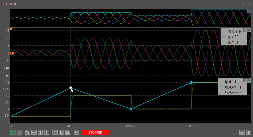
Transients can also be configured graphically. Clicking the preview button or any configurable field switches to the preview mode, provided that a valid transient is defined and that the variable exists in the Scope.
During preview, transient points appear as large dots. Using the mouse, dots can be dragged to set the desired time and amplitude values. To add a new point, double-click near the editable transient signal. To remove an existing point, right-click the point and select the ‘Remove point’ option.
These actions are synchronized with the settings in the right bar. Editing the transient preview does not affect the actual variable until the ‘Fire transient’ button is pressed. To exit the transient preview mode without firing the transient, press the Transient preview button in the right bar again.
Formula Builder
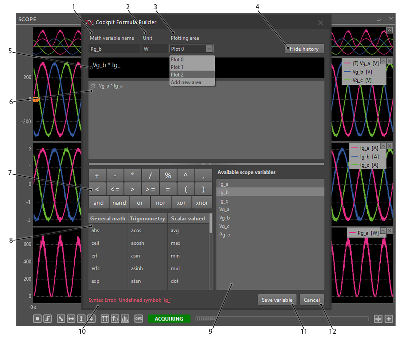
The Formula Builder allows users to create extra mathematical variables for visualization inside the Scope. Any currently displayed variable can be used for that, including analog and digital oversampled data. Mathematical operators and functions provided by the Formula Builder are applied element-wise.
Math variables are calculated by Cockpit once the data is available on the computer, whereas their equivalents in the user code must be computed on the controller. This saves hardware resources and can also be defined more conveniently without recompiling the code.
Interacting with graphs and plots
Managing plot variables
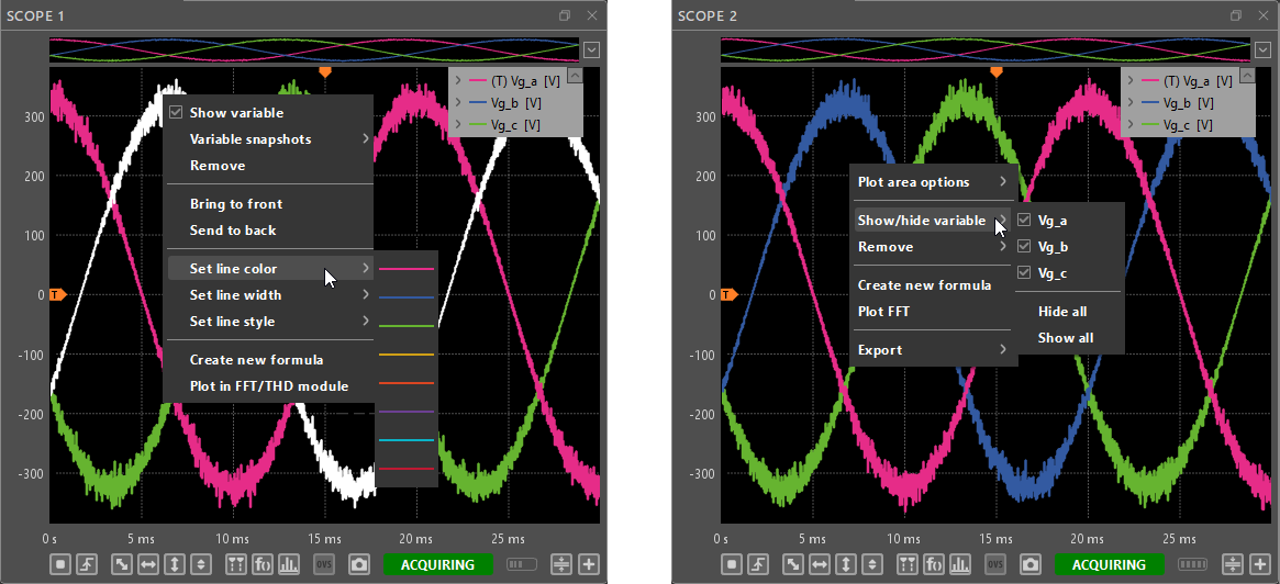
To add a variable to a plot, select it in the USER VARIABLE, ANALOG INPUTS, or DIGITAL I/O section in the project pane, and drag and drop it over the plot. Multiple variables can be selected simultaneously by holding the Shift or Ctrl key. Once added to the Scope, variables also appear in the bottom bar, from where they can be removed or have their visibility changed.
For each variable, most actions can be performed from context menus by right-clicking on a plotted signal.
Managing plot areas
New plot areas can be added by clicking the + button in the bottom-right corner of the module. The total module height can be freely distributed between the plots.
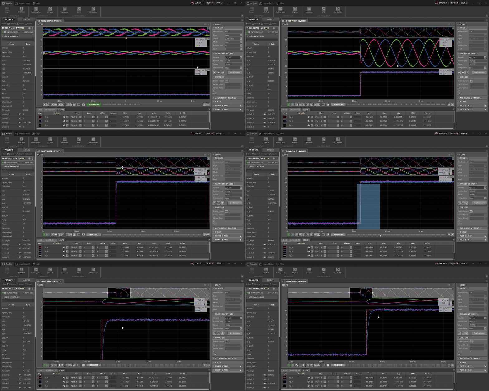
- To zoom in and out along the horizontal axis, place the mouse cursor over the area of interest. Then, use the mouse wheel to zoom in or out at the cursor’s location.
- To zoom in and out along the vertical axis, place the mouse cursor over the area of interest. Then press the Ctrl key and use the mouse wheel to zoom in or out around the location of the mouse cursor.
- To zoom in on a specific area, click and drag to draw a blue rectangle over it.
- To achieve a horizontal auto-scale, right-click and drag horizontally. A light grey horizontal strip will appear. Release the mouse button to perform the horizontal auto-scale.
- To achieve a vertical auto-scale, right-click and drag vertically. A light grey vertical strip will appear. Release the mouse button to perform the vertical auto-scale.
- To enter panning mode, press and hold the middle mouse button or Ctrl + Left mouse button, then move the mouse.
- To prevent a plot from changing the displayed range of values, hover over the y-axis and click the lock icon that shows up. The same can be done from the y-axis pane menu in the right bar.
Scope application examples
The following examples illustrate some use cases of the Scope module:
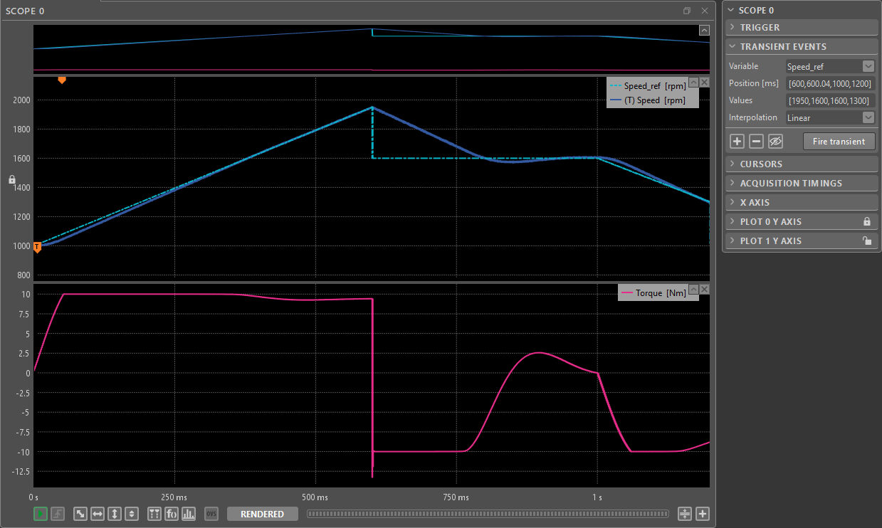
- Measuring the speed tracking performance of an electric motor drive controller.
 By Stéphane Lovejoy • April 12, 2022 • PN300
 By Mateja Ilić • September 12, 2025 • PN303