Table of Contents
This article describes how to use the Scope module of imperix Cockpit to interact with the user code running on imperix power converter controllers, namely the B-Box 4, B-Box RCP, B-Board PRO, the B-Box Micro, and the Programmable Inverter. This page provides a detailed explanation of all of the module’s features.
For new users, it is recommended to read the following articles beforehand to get started with the imperix software development kit (SDK) and imperix Cockpit monitoring software:
Scope module basics
The Scope module allows the user to display control signals on an oscilloscope-like interface by capturing and plotting every sample of the scoped user variables. The acquisition is done at the control task rate (i.e. the main interrupt frequency of the controller), ensuring that each and every sample is scoped.
The scope module can monitor up to 100 MBytes of data. The window length and the control task rate will affect how many user variables can be scoped.
If the control task is set to a standard frequency of 20kHz, it represents scoping one variable for 21 minutes or 32 variables (maximum number of scoped variables) for 40 seconds. On the B-Box 4, up to 64 variables, i.e. 20 seconds of data can be scoped each acquisition.
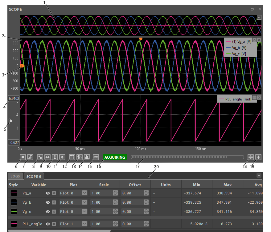
Scope module interface
Advanced scope features
The Scope module offers several advanced features, accessible through the plot footer buttons and the right bar menus.
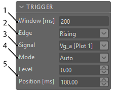
Trigger configuration
The trigger mechanism of the scope module behaves the same way as the trigger on a regular oscilloscope. The Tigger pane located in the right bar allows the configuration of the scope trigger.
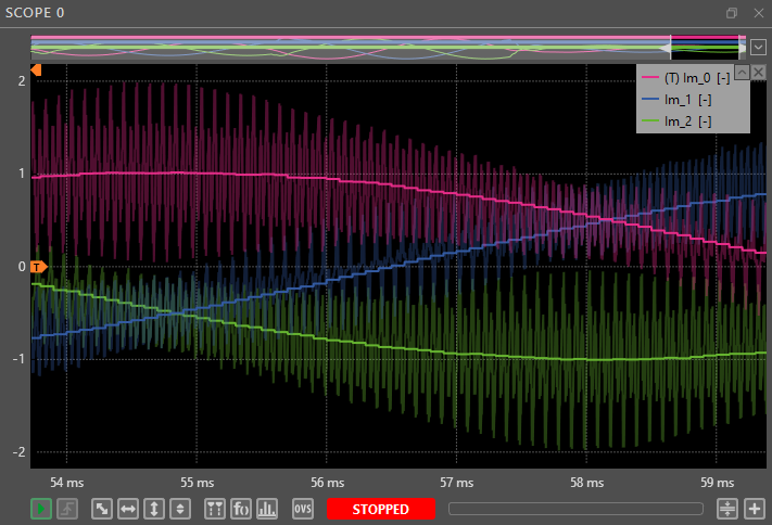
Oversampled signals
Thanks to an upgraded scoping protocol on the B-Box 4, the user can now display data from hardware resource channels directly in the Cockpit Scope Module. These signals are unbounded by the user code control frequency. For example, ADC signals are acquired at the ADC chip acquisition rate of 20 MSps (or 10 MSps if any of the ADC channels 12-23 are used) while PWM signals are acquired with a resolution of up to 4ns.
There are three types of oversampled signals currently available in the Scope:
- ADC channel signals
- Digital I/O (PWM, GPI/O, FLT) channel signals
- Oversampled probes
The first two types of signals can be found below the User Variables list (left bar in Cockpit). They correspond to the channels defined by the ADC, GPI, GPO, FLT and various PWM blocks in the user code. To display them in the Scope, simply drag and drop them like you would any other user variable.
On the other hand, oversampled probes are user variables that are connected directly (or through a constant gain and offset) to an ADC block in the user code. In the Scope, the user can choose to toggle between displaying just the data acquired at the CPU rate and a combination of user variable and ADC channel data.
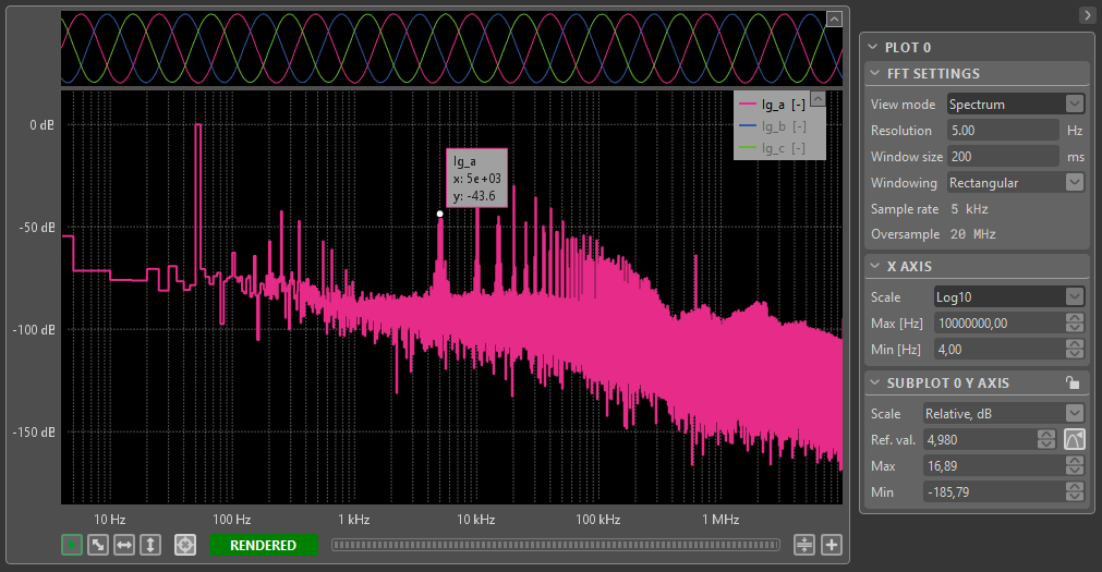
All oversampled signals are compatible with the various metrics calculated in the bottom bar, as well as with the Formula Builder. ADC channel signals and Oversampled probes are also compatible with the Spectral Analyzer, enabling the user to see the spectra of these signals above the Nyquist frequency defined by their control loop rate.
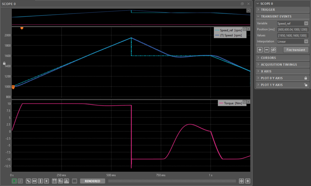
Transient generator configuration
The transient generator allows the user to apply a predefined signal on multiple user variables, provided they are connected to the Tunable parameter block. The signal is defined as a sequence of transient events at different positions within the scope acquisition window.
In the following example, three transient events are applied to Ig_d_ref. It can be seen that these events are generated simultaneously with the acquisition of Ig_a, Ig_b, Ig_c, and Ig_d.
Defining transients graphically
Starting from Cockpit version 2024.3, the transient input signal can be set using an interactive graphical interface. Clicking the preview button or any of the transient event fields causes the transient preview to show up in the scope, provided that:
- The transient events and transient event definitions are valid
- The variable set in the Variable field is added to the Scope
Once the preview shows up, the transient event points, if any are set, will show up as large dots. Using the mouse, the dots can be dragged to set the transient event position and value in one move. To add new points, double click near the editable transient signal and a new dot will show up. To remove existing points, right click on the point and select the ‘Remove point’ option from its context menu.
All of these actions immediately update the corresponding transient event in the right bar. Editing the transient preview does NOT affect the actual Tunable variable or the scope acquisition in any way, unless the ‘Fire transient’ button is pressed. To exit the transient preview mode without firing the transient, simply press the Transient preview button in the right bar again.
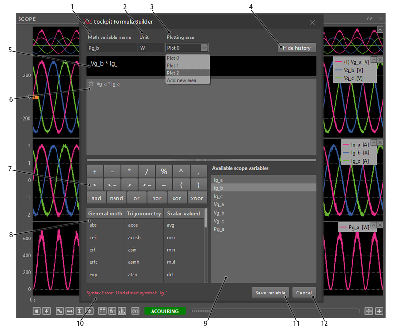
Cockpit Formula Builder
The Formula Builder allows the user to create math variables that are then added to the Scope module. Math variables are created based on a mathematical formula that can include any of the currently Scoped variables.
The math variables are calculated on the PC side after the acquisition of a scope window. This alleviates the need to define every variable to monitor in the user code, saving on hardware resources while still allowing the user to track them live through Cockpit. This also saves time, as new math variables can be added or their formula edited without having to recompile the user code.
With the exception of constant expressions and scalar-valued functions, all of the mathematical operators and functions provided by the Formula Builder are applied element-wise. This means that the formula is applied to each and every sample of the variables included in the expression, creating a new signal to be plotted in the scope.
Scope tips and tricks
- To add multiple variables to a plot, open the user variable section in the project pane.
Keep the ctrl key pressed and click on the desired variables to select them.
Alternatively, click on the first variable to select it, keep the Shift key pressed, and click on the last variable to select. These selected variables can then be dragged and dropped into a plot all at once. - To zoom in and out along the horizontal axis, place the mouse cursor where to zoom. Then, use the mouse wheel to zoom in or out around the location of the mouse cursor.
- To zoom in and out along the vertical axis, place the mouse cursor where to zoom. Then press the ctrl key and use the mouse wheel to zoom in or out around the location of the mouse cursor.
- To zoom on a specific area, click and drag to draw a blue rectangle over the zoom area.
- To achieve a horizontal autoscale, right-click and drag horizontally. A light grey horizontal strip will appear. Release the mouse button to perform the horizontal autoscale.
- To achieve a vertical autoscale, right-click and drag vertically. A light grey vertical strip will appear. Release the mouse button to perform the vertical autoscale.
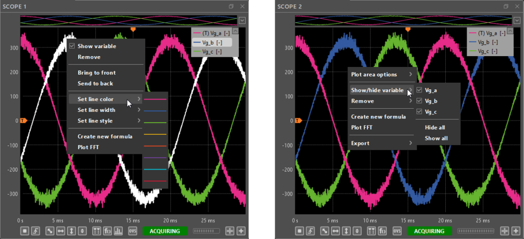
- Many of the Scope functionalities can also be accessed through context menus by right-clicking on a plotted variable or on the empty space in the plots.
Scope application examples
The following examples illustrate some use cases of the Scope module:
- Measuring the speed tracking performance of an electric motor drive controller.