Table of Contents
This article describes how to use the Cockpit System Identification module to interact with the user code running on imperix controllers. This page provides a detailed explanation of all of the module’s features. For users seeking getting-started assistance with Cockpit itself, a separate article is available in PN300.
System Identification module basics
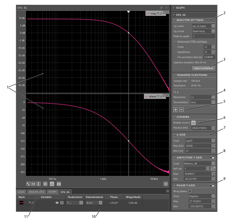
The System Identification (Sys. Id.) module allows the user to launch a system identification experiment and examine the resulting frequency response estimate.
To perform the system identification experiment, the module injects an excitation signal at the control task rate and records the system response. The excitation is a pseudorandom binary sequence (PRBS) signal, and it is injected using the Scope transient generator and the System Identification Injector block.
The data acquired by the Scope is then used by the Sys. Id. module to calculate frequency-response estimates and display their Bode plots. More details on the estimation technique are given in SD041.
Transfer functions in the module are represented by enumerated variables (TF_0, TF_1, TF_2, …). The module always has at least one transfer function variable present (TF_0). The Scope data used to estimate the frequency response for a transfer function variable is selected by setting its numerator and denominator. Any Probe variable defined in the user code can be set as either the numerator or the denominator.
Sys. Id. module interface
Interacting with Sys. Id. module graphs and plots
The Sys. Id. module consists of two plot areas that display graphs of the transfer function variables. This section lists tips and tricks for manipulating plot variables and areas in the module.
Managing plot variables
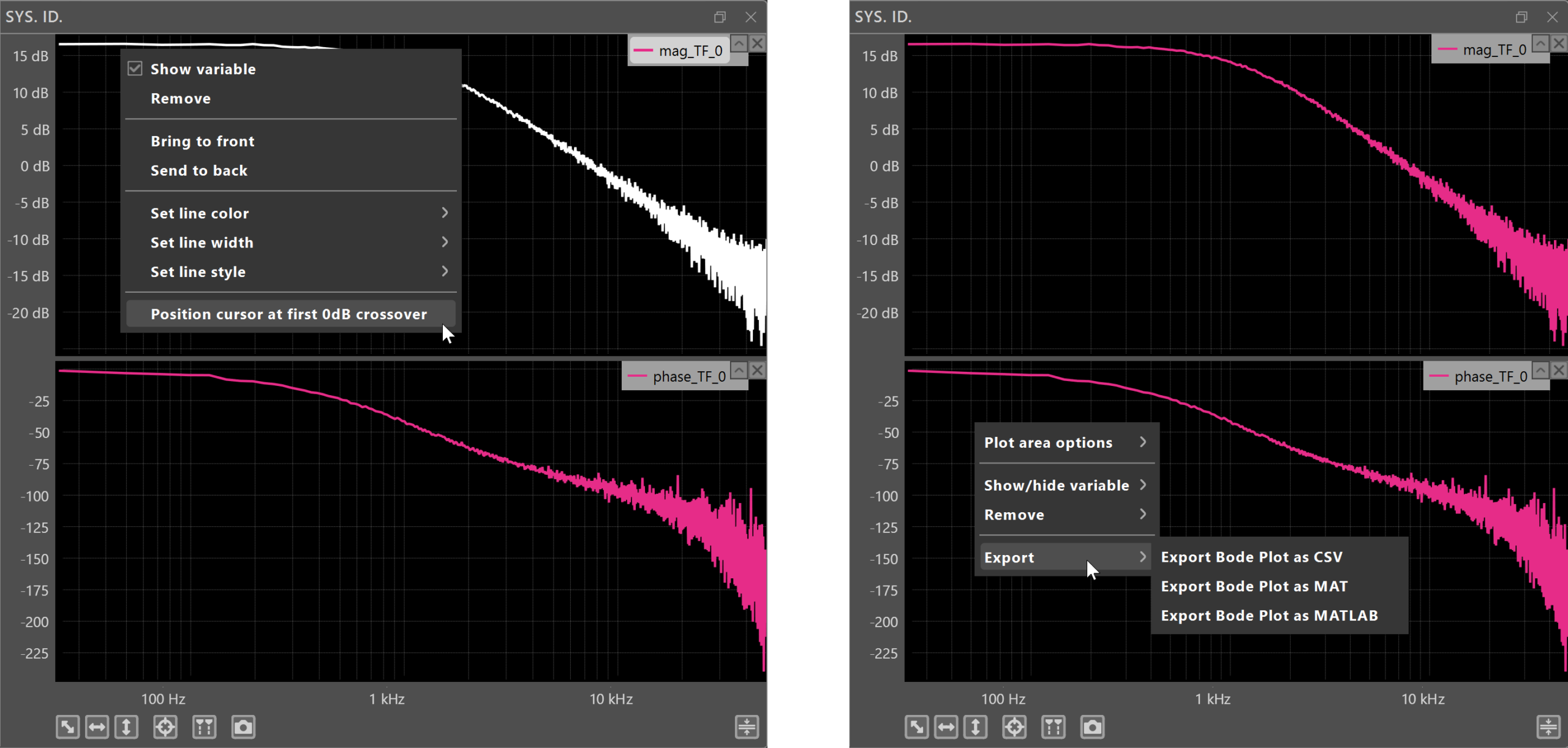
Added transfer function variables will appear as rows in a table in the bottom bar tab for the corresponding module. Here, variables can be removed, and their style, visibility, and plotting order can be managed. If the vertical cursor is enabled, the magnitude and phase values at the cursor position are also shown.
All of these actions can also be accessed from context menus by right-clicking on a plotted variable or on the empty space in the plots.
Managing plot areas
The total module height can be freely distributed between the magnitude and phase plots. To resize plot heights, click on the border between the plot areas and drag.
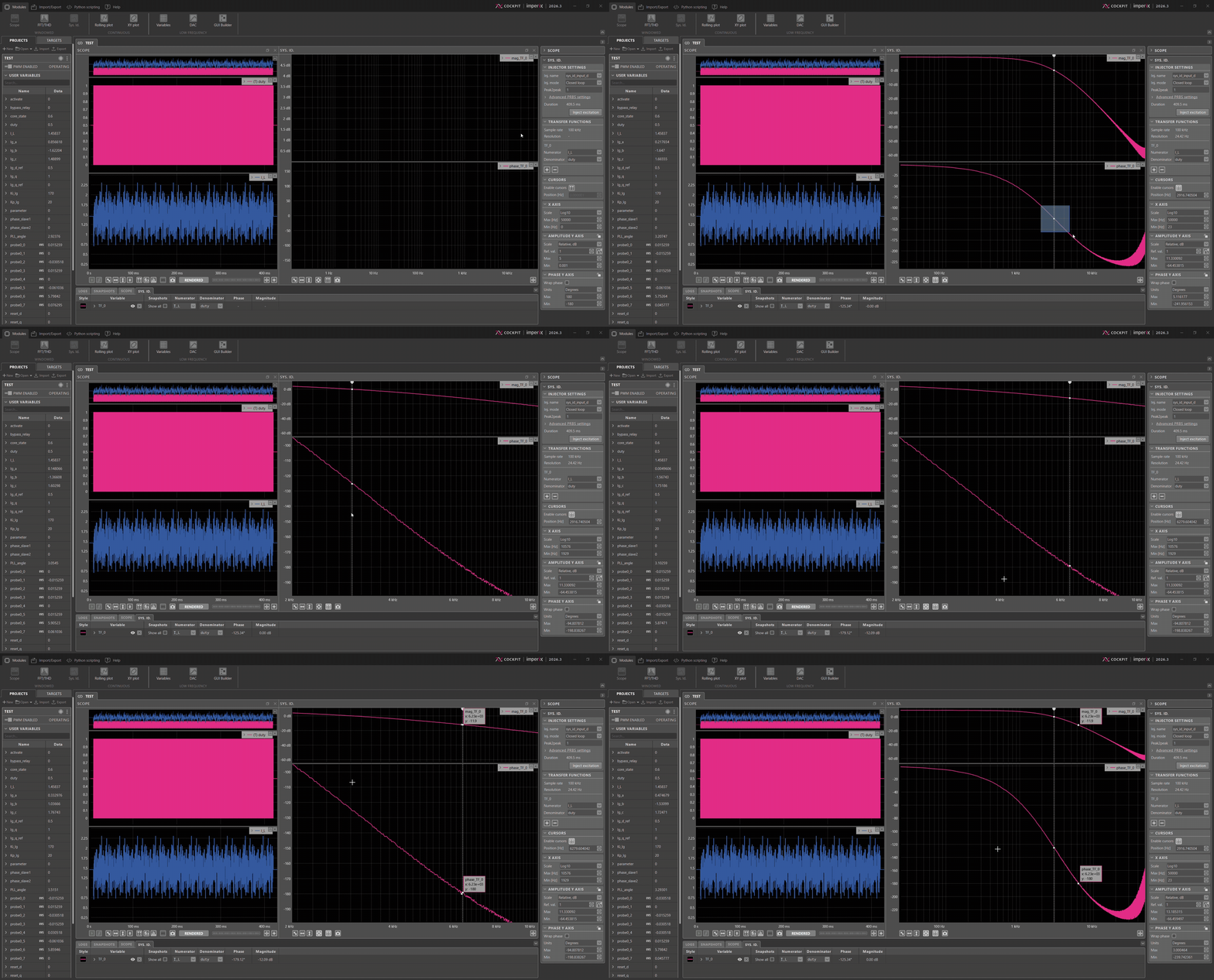
- To zoom in and out along the horizontal axis, place the mouse cursor over the area of interest. Then use the mouse wheel to zoom in or out around the cursor.
- To zoom in and out along the vertical axis, place the mouse cursor over the area of interest. Then press the Ctrl key and use the mouse wheel to zoom in or out around the location of the mouse cursor.
- To zoom in on a specific area, click and drag to draw a blue rectangle over the area you want to zoom in on.
- To achieve a horizontal auto-scale, right-click and drag horizontally. A light grey horizontal strip will appear. Release the mouse button to perform the horizontal auto-scale.
- To achieve a vertical auto-scale, right-click and drag vertically. A light grey vertical strip will appear. Release the mouse button to perform the vertical auto-scale.
- To enter panning mode, press and hold the middle mouse button or Ctrl + Left mouse button, then move the mouse.
- To prevent a plot from changing the displayed range of values, hover over the y-axis and click the lock icon that shows up. The same can be done from the y-axis pane menu in the right bar.
Sys. Id. application examples
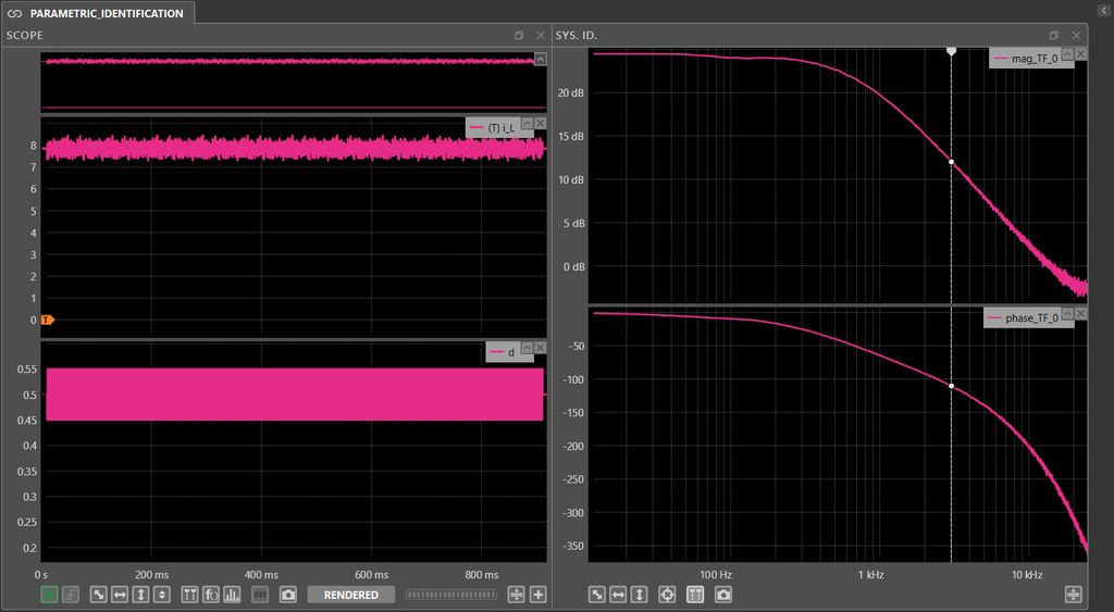
- This example explains parametric identification of a buck converter. Further details are given in PN215.
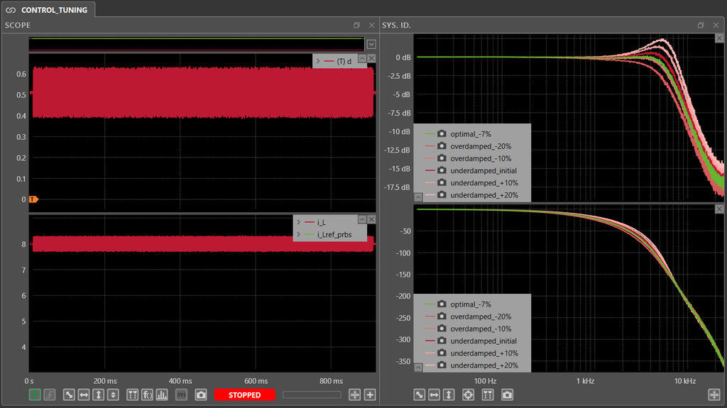
- This example shows how to tune an inductor current controller of a buck converter. Further details are provided in PN216.
 By Stéphane Lovejoy • April 12, 2022 • PN300
 By Mateja Ilić • August 25, 2025 • PN301