Table of Contents
This page is a quick-start guide to build a 3 phase inverter using imperix equipment. It is specifically made to accompany users who want to get familiar with imperix’s solutions and build their first inverter with the B-Box 4 using the Simulink or PLECS blockset. The inverter is built using products included in the power electronics bundle.
The guide focuses on implementing a 3 phase inverter with open-loop generation of sinusoidal currents in a resistive load. The topology of this inverter is shown in Fig. 1. It consists of three half-bridge modules, each connected to an inductor in series with a resistor. These inductors are then connected to the grid connection panel of the power electronics bundle, which is then linked to the resistive load arranged in a star configuration.

Required hardware equipment
The power electronic bundle contains all the required imperix hardware to build a 3 phase inverter. Alternatively, the individual components are listed below. The list comprises imperix products as well as additional components commonly available in power electronic research laboratories:
- Imperix products:
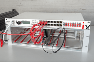
- 1x programmable controller (B-Box 4)
- 3x half-bridge modules
- 1x passives filters box
- Control development tools for Simulink and PLECS (ACG SDK), with a valid license
- Others:
- 3x Resistors (5Ω to 100Ω)
- A DC power supply
- Safety laboratory cables (banana)
- Optional: voltage and current probes with an oscilloscope
Passive components sizing
The circuit is built with 2.2 mH inductors from the passive filter box and 11.5 Ω resistors. Considering the operating conditions of the inverter, a DC bus voltage of 200 V guarantees a maximum output current of 9.2 A with a modulation index of 1. This is confirmed by the formula for the load current from TN152 :
$$I_{RMS}(M = 1) = \frac{1}{\sqrt(2)} \frac{V_{dc}}{\sqrt{(R_{load}+R_g)^2 + (2\pi fL_g)^2}} = 6.12\,\text{A}$$
The output current is therefore well below the 10 A rating of the employed load resistors.
Building and wiring the 3 phase inverter
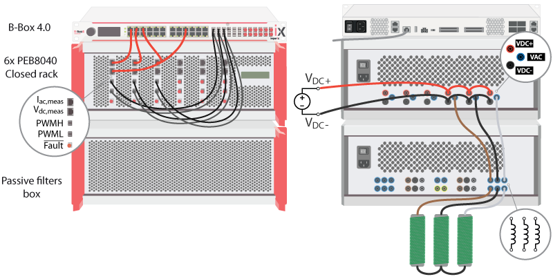
The wiring of the system is done as represented in Fig. 2. The main points to consider are as follows:
- The Ethernet cable is connected to the B-Box 4 so that it can be detected by Cockpit. More information on connecting to the controller is available in PN138.
- Ensure each optical fiber is matched with its designated module and channel.
- The sensors are connected to the designated analog inputs of the controller. Further details on configuring the analog I/Os are provided in the next section.
- The AC output (midpoint, VAC) of the modules is connected to the resistors through the inductor.
- The DC buses of the modules are interconnected, and the DC source is correctly connected by linking DC+ to VDC+ of the modules and DC− to VDC− of the modules.
Analog inputs configuration
Before doing any experiments, it is essential to properly configure the analog input channels of the B-Box 4. These channels have both hardware and software settings. The hardware settings can be configured from Cockpit or the B-Box 4 front panel, and the software settings are configured inside the Simulink or PLECS control model.
Software settings
- Channel number
- Sensor type
- Sensitivity and offset
- Sampling strategy
Hardware settings
- Protection reaction time (e.g. over-current or over-voltage detection)
- Safety limits (upper and lower thresholds)
More information about the ADC block of Simulink and PLECS blocksets can be found here. Additionally, related information on the analog I/O configuration on B-Box 4 can be found in PN252.
The analog channels have been configured as shown in Fig. 3. The limits were computed with a safety margin to prevent unwanted tripping. In this case, no offset was detected. However, if an offset is observed on any channel (i.e., the measured value is different from zero when no signal is applied), the offset should be adjusted. This can be done through the ADC block.
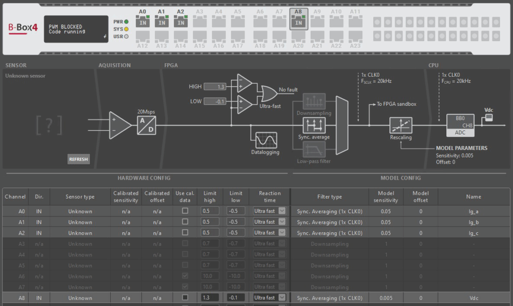
Figure 3. Analog input/output configuration for B-Box 4
Software
Two pieces of software are required to develop the B-Box control code: the imperix Automated Code Generation Software Development Kit (ACG SDK), which can be downloaded here; and a compatible version of Matlab (2016 and newer) or PLECS.
A detailed guide on how to set up the software can be found in PN133.
Creation of the Simulink model
The basic working principles of a 3 phase inverter are explained in TN152. The control model below implements open-loop output-current control. Details on closed-loop current control can be found in TN106. More information on how to create a Simulink or PLECS model are given in PN134 and PN136, respectively.
Simulink model
PLECS model
Generation and real-time execution of the controller code
At last, the code can be built by pressing Ctrl + B on Simulink (Ctrl + Alt + B on PLECS). This will automatically generate and compile the C code that will be uploaded to the B-Box 4. Pressing Ctrl + B also launches the Cockpit monitoring software. Its purpose is mainly to operate the target using tunable parameters and to monitor the inverter through probe variables. Additional details on how to use Cockpit can be found in the Cockpit – User guide.
After creating a new project and linking the user code with the controller, the usre can set up the Cockpit workspace as follows:
- Two different scopes are added to the scope module. The first one will include the three measured currents (
Ig_a,Ig_b,Ig_c) and the second one the duty cycles (d_a, d_b, d_c) and the modulation index (M). - The DC bus voltage (
Vdc) is added to a rolling plot. - The modulation index
(M) variable is added to the variables module.
Once the workspace has been set, the next steps can be followed to run the control:
- Make sure that
PWM switchin the upper left corner of Cockpit is deactivated so that the inverter remains inactive. - Set the inverter modulation index
Mto the value selected for the dimensioning of the load resistors (e.g. leave as 0.8 in the case of the present example). - Gradually increase the DC supply voltage to \(200\,\text V\) (or to the value chosen in the dimensioning of the resistors) and check in Cockpit that
Vdcmatches the voltage of the source. - Enable the PWM pulses in the inverter stage by toggling the
PWM switchin the upper left corner of Cockpit. - Verify that the AC currents
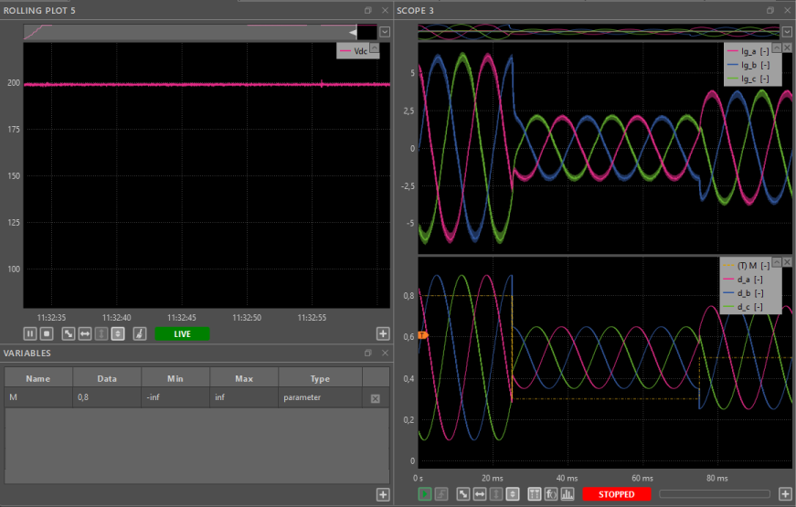
Ig_a,Ig_bandIg_care sinusoidal currents with fundamental amplitude $$\langle\hat{I_g}\rangle=\frac{V_{dc}}{2}\cdot \frac{M_{inv}}{\sqrt{R_g^2+(2\pi f L)^2}}\ \ (\approx 7\,\text A).$$ At this point, the workspace would look similar to Fig. 4. Note that thanks to the new features of B-Box 4, the oversampling currents can also be observed.

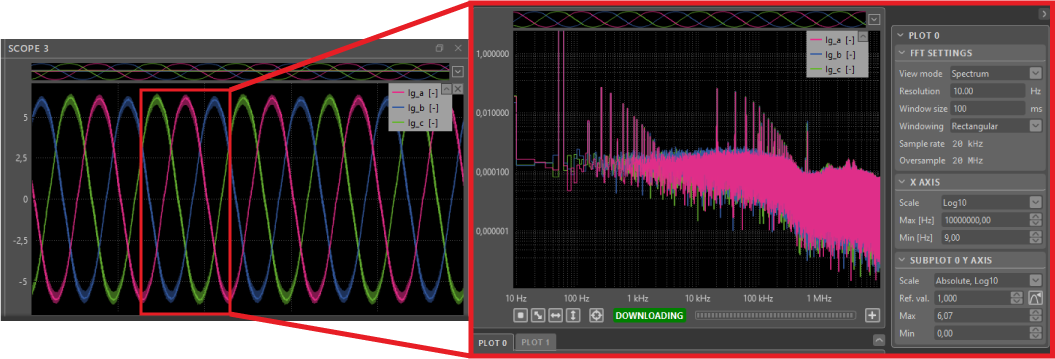
- Use the spectral analyzer in Cockpit to examine the FFT spectrum of the generated currents with a modulation index of
M = 0.8. The obtained results are shown below:
- Generate steps in the modulation index by using the transient generator located in the right-hand panel. Here, the modulation index has a step from
M = 0.8toM = 0.3at instantt = 25ms, and then toM = 0.5att = 0.75ms. The obtained results can be observed in Fig. 6.
- Deactivate the inverter by disabling the PWM pulses with the switch in Cockpit.
- Decrease the DC supply voltage to \(0\,\text{V}\) and observe that the DC-link gets discharged (voltage
Vdcshould decrease to 0).
To go further…
The next step could be to connect the 3 phase inverter to the grid while keeping it connected to the DC source as presented in TN106. As a further step, the DC power supply could be replaced with a photovoltaic panel with a boost stage, to form a three-phase PV inverter for grid-tied applications and showcase the great potential of imperix’s solution for modular power inverters.