Table of Contents
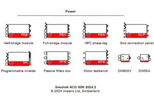
The imperix Power library is a blockset contained within the imperix ACG SDK that provides rapid and accurate modeling of imperix power products. Starting from 2025.1 BETA, the Imperix Power library enables thermal modeling of power semiconductors on imperix power modules. This function is available in Simulink and PLECS. To get started with the Power Library, please refer the Getting-started guide.
This product note summarizes all the useful information on thermal modeling and how to get started with thermal simulation with the Imperix Power library. A simulation example of a Buck converter with a PEB8038 half-bridge module is provided to show how the thermal simulation model is established and validated in experiments.
• ACG SDK 2024.2: First release. Support for PLECS and Simulink SPS library (“Black” blocks).
• ACG SDK 2025.2: Addition of thermal models for most PEB and PEN modules.
• ACG SDK 2026.1: Support for the latest products (PEB-800-40, VSR-1000-ISO, VSR-500-HBW, CSR-25-HBW).
• ACG SDK 2026.1.3: Support for Simulink Simscape Electrical library (“Blue” blocks).
• Simulink (R2016a or newer): Simscape is required.
• Plexim PLECS (4.5 or newer): No particular requirement.
Additionally, for Simulink:
• Simscape Electrical library: Simscape Electrical is required.
• SPS library: Simscape Specialized Power Systems (up to R2025b) or OPAL-RT SPS Software is required.
Thermal models are currently unavailable in Simscape Electrical library.
Introduction
Why thermal modeling is useful
Power semiconductors, such as MOSFETs, IGBTs, and diodes, generate conduction and switching losses during their operation. For power electronics engineers, thermal modeling of power semiconductors provides a way of evaluating the impact of different control and modulation strategies (for example, Carrier-based PWM and Space Vector PWM) on losses via simulation. By linking electrical control strategies to thermal outcomes, engineers can better test and optimize the efficiency of their systems.
Thermal modeling is useful in many power electronics applications. For example in Electric Vehicles (EVs), thermal simulation helps to estimate the losses in inverters under varying torque and speed profiles, and guides the design of thermal management. In micro-grid systems, thermal simulation is useful in optimizing the controller and modulation of multi-level converters, enhancing the efficiency of power delivery.
Several semiconductor manufacturers provide dedicated simulation tools or models for their components. PLECS and Simscape also provide their thermal simulation libraries. For the users of imperix power modules, the Imperix Power library provides rapid and accurate thermal modeling of semiconductors in offline simulation based on PLECS and Simulink.
How to use Imperix Power library for thermal simulation
As of today, the Imperix Power library includes the thermal simulation models for PEB8038, PEB8024, and PEN8018, covering most of the power applications using imperix power modules. More thermal models will be included in the future release.
Before starting to use the Imperix Power library for thermal simulations, it is strongly recommended to read the PN150 first, which introduces the basics of the Imperix Power library.
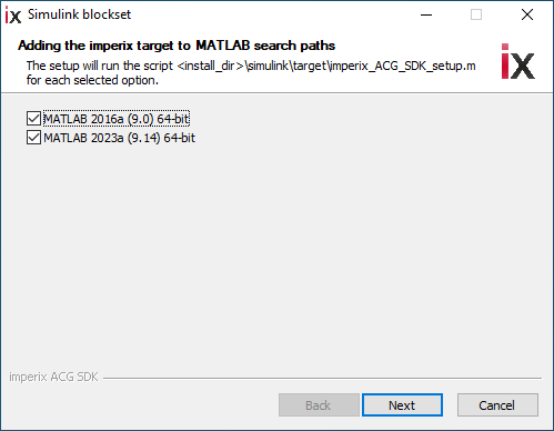
The Imperix Power library is included with the ACG SDK. To enable thermal simulation, thermal description files must be added to the path of the simulation software (Simulink or PLECS). In Simulink, these files are automatically added by the script imperix_ACG_SDK_setup.m during the installation of ACG SDK (see below). If the script was not executed during installation, it can also be executed manually from the MATLAB Command Window.
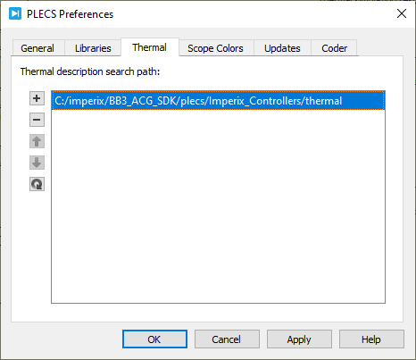
In PLECS, the thermal description files must be added manually. Users must open PLECS and go to Files -> PLECS Preferences -> Thermal tab and add <install dir>/plecs/Imperix_Controllers/thermal into the thermal description search path. Once done, all the thermal description files can be viewed in Window -> Thermal Library Browser.
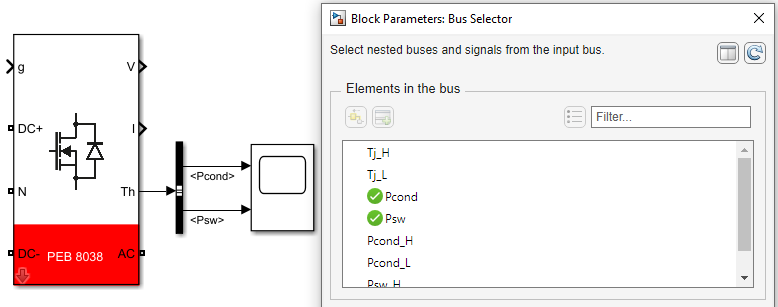
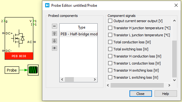
Thermal simulation can be enabled in the Thermal Tab of a mask in Simulink or PLECS. All the losses are averaged over a chosen period, which is 1 ms by default. The thermal simulation results can be acquired through the Th bus output in Simulink or a probe in PLECS.
Thermal modeling of imperix power products
The thermal modeling of an imperix power product mainly focuses on the modeling of the semiconductors. The losses generated outside the semiconductors are ignored, such as the DC-link and the PCB traces. In addition, the variable speed of the fan on the heatsink is not modeled, and full speed is always considered. Overall, the established thermal model consists of two parts, namely:
- Modeling of the thermal losses of power semiconductors. For switching devices such as MOSFETs and IGBTs, the switching loss (turn-on and turn-off loss) and conduction loss are modeled. For diodes, the reverse recovery loss (turn-off loss) and conduction loss are modeled.
- Modeling of the thermal impedance network between the semiconductors and the air, including the thermal resistance and thermal capacitance.
It is important to mention that only the thermal resistance is modeled in the Imperix Power library blocks. All the thermal capacitances are either ignored or fixed at a small value to reduce the simulation time for the system to reach a thermal steady state. Therefore, the imperix Power library is mainly aimed at simulating the losses and temperatures in the steady state, but it cannot accurately simulate the dynamic changes of temperature when the operating condition changes.
The losses of power semiconductors vary under different operating conditions. More specifically, the conduction loss is modeled by the drain-to-source on resistance \(R_{DS(on)}\) (for MOSFET) or forward voltage \(V_{f}\) (for IGBT and Diode), which depends on the on-state current and temperature. The switching loss depends on the device current and voltage during the switch transient, which is however difficult to simulate accurately. A more practical method is to read the operating conditions from an ideal electrical model and get the losses based on prebuilt look-up tables provided by the manufacturers. The detailed implementation method is different in PLECS and Simulink and will be addressed separately in the subsequent sections.
PLECS
PLECS records the semiconductor’s operating condition (forward current, blocking voltage, junction temperature) before and after each switch operation. It then uses these parameters to read the resulting dissipated energy from a look-up table. [1] The turn-on loss \(E_{on}\) and turn-off loss \( E_{off} \) are modeled by a 3D look-up table as shown in the following example. The \(E_{on}\) is represented as pulses that only take value at switch-on events, and have to be averaged over a certain period to get the turn-on loss \(P_{on}\) in watt. Same for the turn-off loss \(P_{off}\).

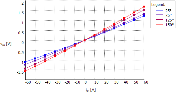
The semiconductor’s drain-to-source voltage at on state \(V_{on}\) is modeled by a 2D look-up table as shown below. The conduction loss \(P_{cond}\) is then calculated by \(P_{cond} = V_{on} \cdot I_{on}\).
Several manufacturers provide thermal modeling files of their power semiconductors or modules [2], while the implementation method varies among different manufacturers. In the Imperix Power library, all the power semiconductors are modeled with ideal devices, and the body diodes of MOSFET and anti-parallel diodes of IGBT are also modeled separately. The look-up tables are taken from the manufacturers’ files.
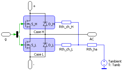
The thermal resistance between the semiconductor’s junction and the case is also provided by the manufacturers, while the thermal capacitance is either ignored or fixed at a small value (0.01 J/K usually) for the reason previously explained. To complete the thermal network, the thermal resistance between the heatsink and the ambient temperature is measured experimentally. Finally, the thermal simulation model of an imperix power product is obtained, as shown below. Note that each Heat Sink block represents the case of a semiconductor component.
Simulink
The Simscape Electrical library includes thermal models of semiconductors and a loss visualizer, which features a different implementation approach to model power losses from PLECS. This page will focus on the implementation using Specialized Power Systems.
Unlike PLECS, the Simscape Specialized Power Systems library doesn’t have a built-in method for the thermal modeling of semiconductors. However, this functionality can be implemented by recording the operating conditions from the electrical model and calculating the losses based on the look-up tables provided by the manufacturers.
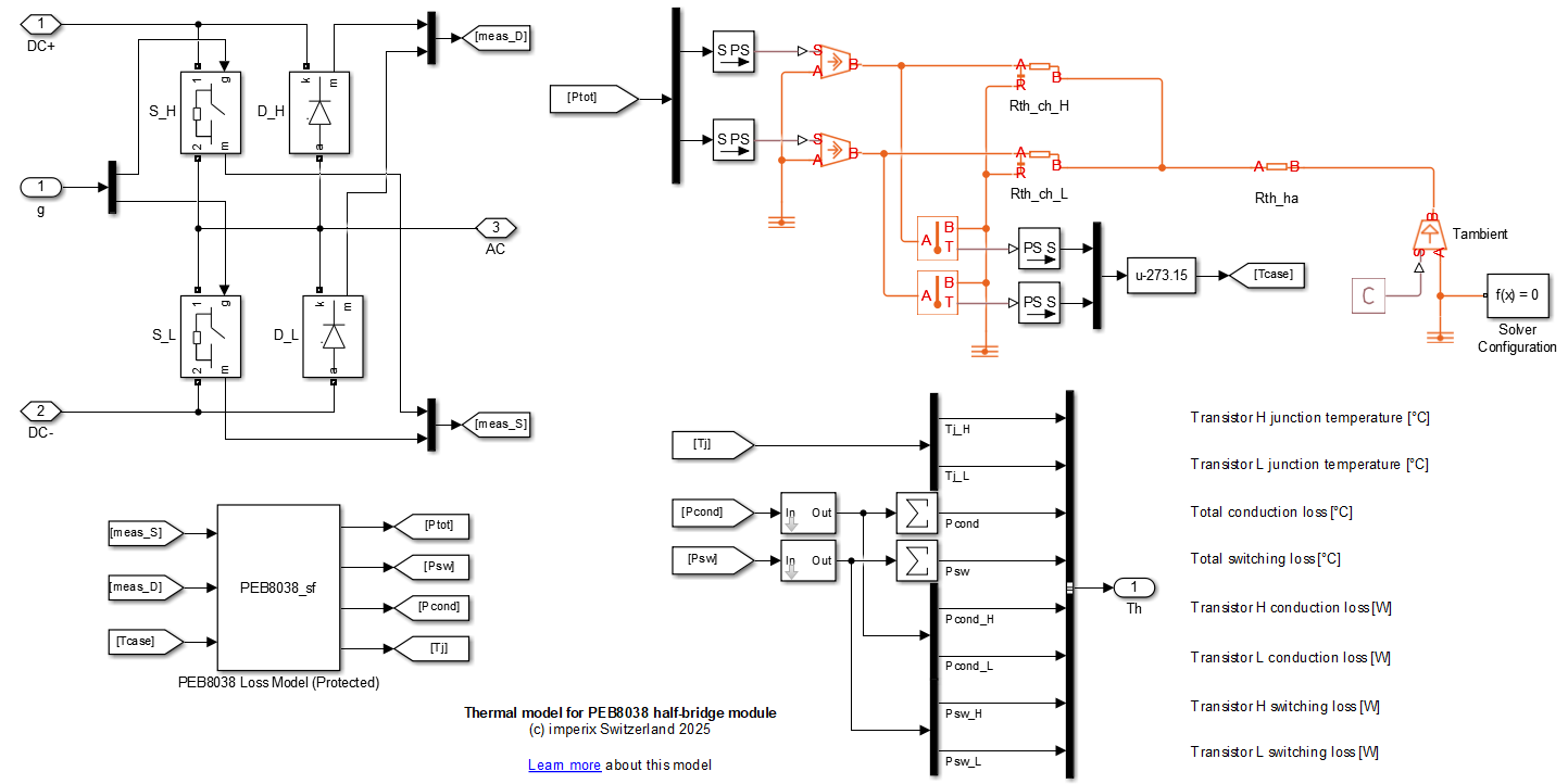
The thermal model, including the thermal impedance network, is built with the Thermal sublibrary of Simscape. Semiconductors are modeled as controlled thermal sources, linking the electrical domain and the thermal domain. The thermal simulation model is obtained in Simulink, as shown below.
Reference
[1] Plexim, “Thermal Simulation”, https://www.plexim.com/products/plecs/thermal, Accessed Dec. 2024.
[2] Plexim, “Thermal Semiconductor Models for PLECS”, https://www.plexim.com/download/thermal_models, Accessed Dec. 2024.
Experimental validation of the loss model
As previously explained, the established thermal models include the semiconductor’s loss model and the thermal impedance network model. However, it is hard to validate the impedance model experimentally because the junction temperature is inaccessible. Therefore, this page will focus on the validation process of the loss model. A two-step experiment is designed to compare the total losses between the simulation and experiment under different operating conditions.
In the first step, the relationship between a module’s total loss \(P_{tot}\) and the temperature rise \(\Delta T\) of the heatsink is modeled, which provides an indirect measurement of the losses by measuring the heatsink temperature. Meanwhile, the thermal resistance between the heatsink and the ambient temperature is also measured in this step. In the second step, the same module is operated under different working conditions, and the measured total losses are compared with the simulation results.
This page introduces the experimental validation of the PEB8038 model as an example, with the simulation model provided in Simulink and PLECS. A similar process can be applied to PEB8024 and PEN8018 as well.
Measurement of thermal losses
The total loss \(P_{tot}\) generated by the semiconductors of a power module is indirectly measured by measuring the temperature rise \(\Delta T\) at a fixed point on the module’s heatsink.
As the following circuit diagram shows, the first-step experiment is performed to model the relationship between \(P_{tot}\) and \(\Delta T\). The module under test is supplied by a DC source working in constant current output mode. The two gates are switched ON simultaneously. In this case, the total loss \(P_{tot}\) is equal to the conduction loss \(P_{cond}\), which can be calculated by \(P_{cond} = V \cdot I\), where the current \(I\) is measured by the voltage drop on a 10mΩ shunt resistor, and the voltage \(V\) is measured by a multimeter.
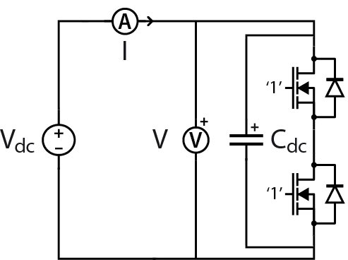
The heatsink’s temperature \( T\) is measured by a temperature sensor glued on it. Another temperature sensor is put aside to measure the ambient temperature \(T_{amb}\). During the test, the fan on the heatsink always runs at full speed. By increasing the DC current and recording the temperature, an equation between the total loss \(P_{tot}\) and temperature rise \(\Delta T = T – T_{amb}\) is acquired. The following figure shows a good linear relationship between the two.
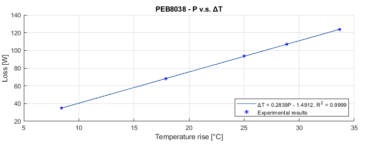
Furthermore, this figure also validates the fact that the module’s heatsink can be modeled with a thermal resistance, whose value equals the slope of the line, which is 0.2839 K/W. With this curve, the module’s total loss \(P_{tot}\) can be calculated by applying the measured heatsink temperature rise \(\Delta T\) to the equation.
Comparison between simulation and experimental results
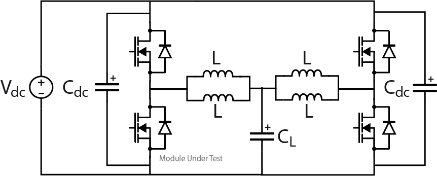
The circuit diagram of the 2nd-step experiment is depicted below. The module under test works as a Buck converter with a fixed duty cycle. A 50% duty cycle is chosen for the experiment listed below, but other values could also be selected and the same conclusion would be achieved. Another PEB8038, working as a Boost converter with a PI current controller, is used as a current-controlled load. The DC bus is supplied by an 800V DC source. The load capacitor \(C_L\) is 10µF, and each inductor \(L\) is 2.2mH.
The simulation models in Simulink and PLECS are provided below. Due to the different implementation methods of the thermal model, the simulation results can be slightly different between Simulink and PLECS (1-2 watts at max in terms of total losses), which doesn’t affect the conclusions. Note that all the results given below are based on the PLECS model.
Simulink model
PLECS model
The second-step experiment is performed by running the system in different currents and switching frequencies. The DC bus voltage is kept at 800V throughout the experiment. By measuring the temperature rise \(\Delta T\) at the same measurement point on the heatsink as the first step, the module’s total loss \(P_{tot}\) can be calculated with the obtained equation, and the simulation and experimental results are compared in the graph below.
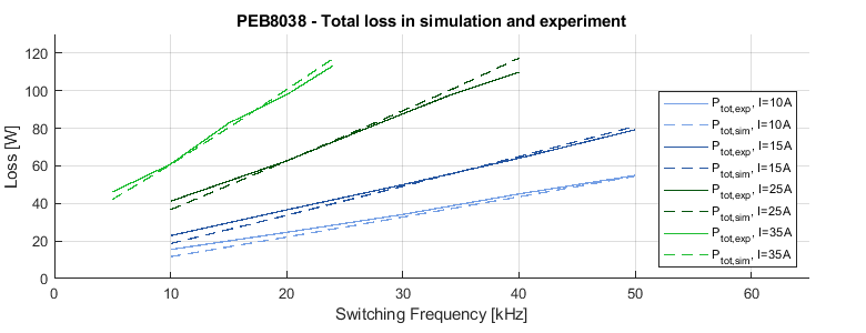
Overall, the simulated total losses are generally consistent with the total losses measured in experiments. The difference may come from inaccuracies in the measuring tools, especially the temperature measurements. Moreover, although the effect of gate resistance has been taken into account in the manufacturers’ models, the switching characteristics in the PEB module may still differ from the manufacturers’ test environment due to different gate drivers and parasitic capacitances.
Further analysis is possible based on the thermal simulation results. Due to space limitations, not all the data under all the operating conditions is listed. It can be observed that the simulated conduction loss is approximately proportional to the current, while the switching loss is approximately proportional to the switching frequency, which is expected.
| fsw [kHz] | Ptot,exp [W] | Ptot,sim [W] | Pcond,sim [W] | Psw,sim [W] | Tj,H [°C] | Tj,L [°C] |
| 10 | 15.47 | 11.66 | 2.28 | 9.38 | 37.94 | 32.69 |
| 20 | 24.63 | 22.12 | 2.44 | 19.67 | 47.19 | 36.15 |
| 30 | 34.14 | 32.77 | 2.68 | 30.09 | 56.59 | 39.70 |
| 40 | 45.06 | 43.56 | 2.93 | 40.63 | 66.20 | 43.41 |
| 50 | 54.92 | 54.56 | 3.19 | 51.36 | 75.82 | 47.08 |
To go further
The same simulation model can also be used for the validation of PEB8024. A three-phase grid-connected NPC converter model is used for the validation of PEN8018, and the simulation models are given below.
Simulink model
PLECS model
For more details on the thermal models, please read the dedicated software documentation pages.
More power library examples are available on the Knowledge Base, covering a wide range of application scenarios.