Getting started with Imperix Power library

This article summarizes useful information for getting started with the Power library and provides an example that simulates a three-phase PV inverter.

More general information about getting started with the ACG SDK is given in PN134.

What is the Imperix Power library?

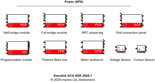
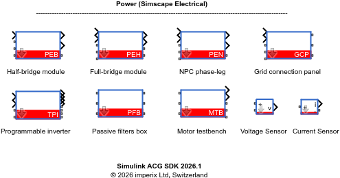
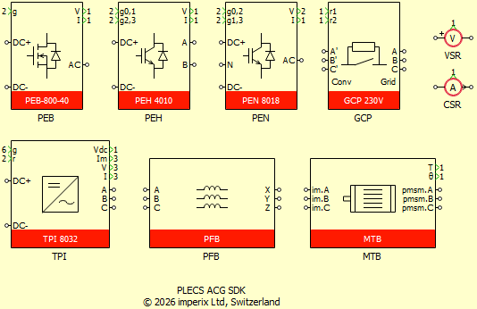
The imperix Power library regroups three blocksets that include accurate simulation models of imperix power products. It comprises nine blocks that foster practicality and accuracy for developing the plant model during offline simulation.

The library supports Simulink and PLECS, with only minor software-dependent differences between the two environments. Since release 2026.1.3, two blocksets are available for Simulink, namely a library specific to Simscape Electrical (blue blocks), and a separate one for Specialized Power Systems (up to 2025b) or OPAL-RT SPS Software (since 2026a).

Imperix blockset	Supported software	Compatible solver(s)
SPS library	Simulink (2016a to 2026a)	– Mathworks’ Specialized power systems (up to Simulink 2025b). – Opal-RT’s SPS software.
Simscape Electrical library	Simulink (2016a to 2026a)	– MathWorks’ Simscape Electrical.
PLECS	PLECS (4.5 or above)	PLECS (any)

Content of the power library

The Power library contains simulation models for all imperix products, classified per circuit topology. For instance, all the half-bridge power modules are included in one PEB block with optional variants PEB-800-40, PEB 8038, PEB 8024, and PEB 4050.

Product name	Block name	Variants
Half-bridge module	PEB	PEB-800-40, PEB8038, PEB8024, PEB4050
Full-bridge module	PEH	PEH2015, PEH4010
NPC Phase-leg	PEN	PEN8018
Grid connection panel	GCP	AC 230V, AC 110V
Programmable inverter	TPI	–
Passive filters box	PFB	–
Motor testbench	MTB	–
Voltage sensor	VSR	VSR-1000-ISO, VSR-500-HBW, DIN800V
Current sensor	CSR	CSR-25-HBW, DIN50A

Modeling levels

By essence, modeling a system requires identifying its relevant physical characteristics and involves making some simplifying assumptions. These choices often depend on the intended purpose and the required level of correctness or relevance. In general, in computer simulation, a trade-off must be made between complexity and accuracy, because more detailed models often come at the cost of slower simulation times.

Due to the above considerations, each block offers two modeling levels, mostly distinguished by how the frequency-dependent behavior of each circuit is modeled:

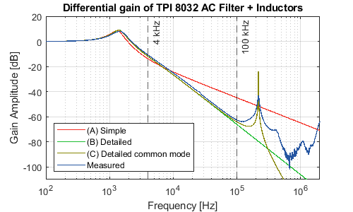
• (A) Simple is a simplified plant model that only considers the main circuit components. Frequency-dependent characteristics above typically 4kHz are ignored to achieve faster simulation speed. This level is well suited for system-level modeling and/or for the simulation of slow control loops. Some models only have the Simple level available, such as GCP and MTB.
• (B) Detailed ensures higher modeling accuracy at the cost of increased simulation time. Frequency-dependent characteristics are relevant up to approximately 100kHz. This level is well suited for circuit-level modeling when higher accuracy is required.

Both modeling levels only take differential-mode characteristics into account. This is because common-mode characteristics generally lie in the higher part of the frequency spectrum, above the considered range of interest. However, an exception is made in the TPI model, which provides an extra modeling level:

• (C) Detailed common mode also encompasses relevant phenomena up to about 100 kHz. However, unlike (B) Detailed, it also models the common-mode feedback path between the AC EMC filter and the DC bus. A detailed explanation of why this is relevant is given on the dedicated software page: TPI block.

Modeling of power circuits

All power circuits are modeled with frequency-dependent characteristics, mostly influenced by their DC bus capacitors (and the inductors/filters when present). As an illustration of the difference between the modeling levels, the figure below shows the transfer function of the TPI model compared with measured results:

It is important to distinguish the frequency validity range, where the simulation model is reasonably close to reality, from the control or switching frequencies. In fact, it is usually not necessary for the converter control and switching frequencies to fall within the plant model’s frequency validity range. For instance, most of the examples available on the knowledge base provide sufficient accuracy with the Simple level, and yet implement control and PWM operation at 20kHz.

Modeling of sensors

Sensors are modeled either as an ideal measurement circuit, or a first-order low-pass filter (LPF). The relationship between sensor’s bandwidth \(f_{BW}\) and the time constant \(\tau\) of the LPF follows \(\tau = \frac{1}{2\pi f_{BW}}\).

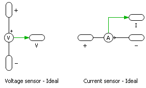
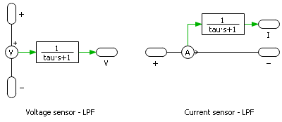
Inside the Power library, a sensor is modeled as a first-order LPF only if its bandwidth lies within the frequency range of a given modeling level. Otherwise, it is modeled as an ideal sensor.

Sensor	Bandwidth [kHz]	(A) Simple	(B) Detailed
VSR-1000-ISO	100 / 10	Ideal	LPF
VSR-500-HBW	3000 / 300	Ideal	Ideal
DIN800V	100	Ideal	LPF
CSR-25-HBW	1500 / 150	Ideal	Ideal
DIN50A	200	Ideal	Ideal
PEB8024, PEB8038, and PEB4050 voltage	8	Ideal	LPF
PEB8024, PEB8038, and PEB4050 current	280	Ideal	Ideal
PEB-800-40 voltage	10	Ideal	LPF
PEB-800-40 current	75	Ideal	LPF
PEH voltage	25	Ideal	LPF
PEH current	120	Ideal	Ideal
NPC voltage	25	Ideal	LPF
NPC current	450	Ideal	Ideal
TPI DC voltage	10	Ideal	LPF
TPI module current	360	Ideal	Ideal
TPI AC voltage/current	200	Ideal	Ideal

Transistor model type

The Power library offers two options for modeling the power transistors:

• Switched: The power transistors are modeled by individual switches. Their control inputs are instantaneous logical gate signals.
• Averaged: The switches are modeled by controlled voltage and current sources. Their control inputs are the relative on-times of the transistors with values between 0 and 1. The gate signals can be either instantaneous (using only values 0 and 1) or time-averaged.

Although the functionality is essentially the same, these options are named differently in PLECS and Simulink/Simscape to align with their respective naming conventions.

This option is available only for models that contain power transistors, including PEB, PEH, PEN, and TPI. In particular, the PEN block in Simulink only has the Switched model.

How to use the Imperix Power library?

Typical use case scenarios

Typical use cases of the Imperix Power library are shown below. These represent a reasonable trade-off between accuracy (in the broad sense of the word) and simulation speed. Please note that this table is more of a recommendation than a hard limit.

Typical use case	(A) Simple Preferable for power system users	(B) Detailed Preferable for power electronics users	(C) Detailed common mode Only available in TPI
(A) Switched Preferable in switch-level simulation	• Voltage / current control at low frequency, typically 20kHz or below; • Phase modulation;	• Voltage / current control at high frequency; • Filter resonances;	• TPI AC precharge; • Space-Vector PWM; • Harmonics injection;
(B) Averaged Preferable in system-level or HIL simulation	• Power flow control; • Energy management; • System-level operation (energizing, discharge, state machines); • Primary, secondary, and tertiary control;	/	/

Use the averaged model with duty-cycle output from PWM blocks

The Averaged mode can also accept duty-cycle inputs between 0 and 1. In this case, the PWM modulator can be removed from the simulation model, significantly reducing simulation time. To use this feature, open the CB-PWM block in Simulink or PLECS, and find the Simulation output type option.

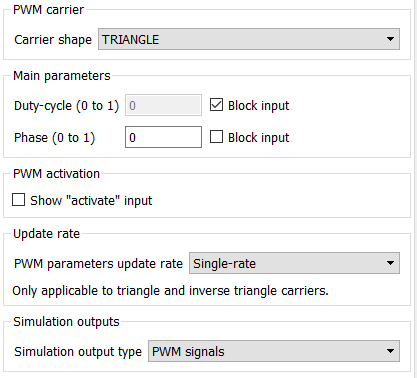
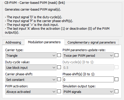
When the simulation output type is set to Duty-cycle, the output of the CB-PWM block will be updated at the end of each controller step, and the PWM phase will be ignored. Therefore, this option is not suitable for phase modulation techniques, such as TN115.

Global configuration of the blocks

The Modeling level and Transistor model type options can be set individually for each block. However, for a large plant model with numerous blocks, a global configuration for all the blocks is usually preferred. The global configuration is available in both Simulink and PLECS.

Simulink

In Simulink, the global configuration of the Power library blocks is managed by the CONFIG block. The detailed procedure is as follows:

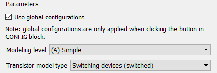
1. In the Simulink model, open the block where the global configuration is to be applied. Tick the box Use global configurations. Note that the global configuration will apply only to blocks with this box ticked. The other blocks will have their local configuration unchanged.

2. In the Simulink model, open the Config block, go to the Power library tab, and select the appropriate options for Modeling level and Transistor model type. As the averaged model is usually used together with the duty-cycle outputs from the CB-PWM blocks, the simulation output types for CB-PWM and TPI CB-PWM are also configured globally here.

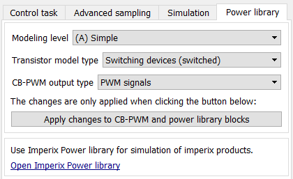
3. Click on the button to apply changes to CB-PWM and power library blocks. The changes will be applied only when the button is clicked and not automatically updated each time at the beginning of the simulation.

PLECS

In PLECS, the global configuration can be easily controlled by a global variable using the <reference> option in the masked block. The detailed procedure is as follows:

1. In the PLECS model, open the Simulation parameters window (Ctrl + E) and go to the Initialization tab.
2. Define two variables modeling_level and transistor_model_type in the Model initialization commands, so that these two variables will be initialized during compilation. The values of these two variables are as follows:

Variable	= 1	= 2
modeling_level	(A) Simple	(B) Detailed
transistor_model_type	Switched	Sub-cycle average

3. Open the PLECS block where the global configuration is to be applied, choose <reference> for Modeling level and Model of power module options, and then put the two variables inside.

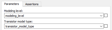
4. Change the values of the two variables to apply a different global configuration. The changes will be automatically applied each time at the beginning of the simulation.

Troubleshooting

This section summarizes some possible issues and solutions when using the Imperix Power library.

Powergui settings in Simulink

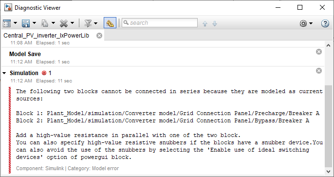
As introduced in PN135, whenever possible, it is recommended to use a Continuous plant model for an accurate and efficient simulation. Exceptions to that are indicated in TN182 for increasing the simulation speed with Simscape Electrical. It is also recommended to tick the box Use ideal switching devices. Otherwise, Simulink may report an error when simulating the relays included in the TPI and GCP blocks.

Initial states in Simulink

For the blocks including DC bus capacitors, the initial voltage across the DC bus can be defined from the block mask. However, when multiple DC bus capacitors with different initial voltages are connected in parallel, Simulink may report a warning about an initial state conflict. This warning usually occurs when simulating with the (A) Simple modeling level, and indicates a structural incompatibility because voltage sources of different values are short-circuited.

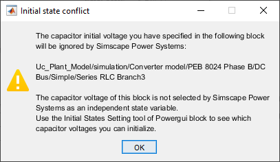
The initial state conflict will not affect the simulation results as long as all DC bus capacitors connected in parallel have the same initial voltage. However, it can be quite annoying to see these pop-up windows at the beginning of each simulation. Unfortunately, there is no good way to actively hide this warning message. As a possible workaround, the initial state conflict can be resolved by simulating the ESRs of DC bus capacitors using (B) Detailed modeling level.

Sensor sensitivity in PLECS ADC blocks

Starting from ACG SDK 2024.2, the ADC and TPI ADC blocks in PLECS have the option to Simulate sensor(s) sensitivity(ies). If this option is ticked, the ADC block expects its input to be the physical value of a sensor’s output, and the reciprocal of the sensor sensitivity is applied to the data flow to get the true value in the circuit.

For simulation, the sensor sensitivity is mostly irrelevant. It is far more convenient to ignore the sensor sensitivity and use true values everywhere. As such, all Power library blocks have the real values as block outputs. As such, when using the Imperix Power library with PLECS ADC blocks, the Simulate sensor(s) sensitivity(ies) tickbox should be selected.

On the other hand, the sensor sensitivity can be useful for Hardware-in-the-loop (HIL) simulation, when the true values must be scaled to the simulator’s analog output range. In this case, a PLECS Probe block can be used to get the sensor output values. For that, drag the Probe block from the PLECS library into the model that contains the circuit. Double-click the icon to open the probe editor window, then drag the Imperix Power library blocks into it as shown below.

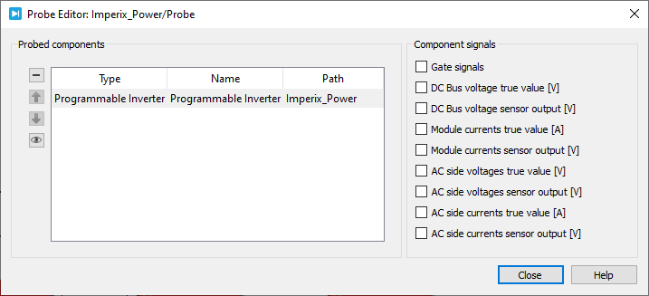
In the next section, a PLECS model example is provided to show how to deal with the true values and sensor outputs when using the Imperix Power library.

State/source dependence issue

As introduced in this note from Plexim, Simulink and PLECS report the state/source dependence issue when a capacitor is directly in parallel with a voltage source, or an inductor is directly in series with a current source.

When using the Imperix Power library, this problem usually happens when the plant model contains a power module block directly connected to a DC source. This is because the Simple level ignores the Equivalent Series Resistance (ESR) of the DC Bus capacitors. For example, in a plant model of a Buck converter, an error message appears if the PEB block is set to the Simple level.

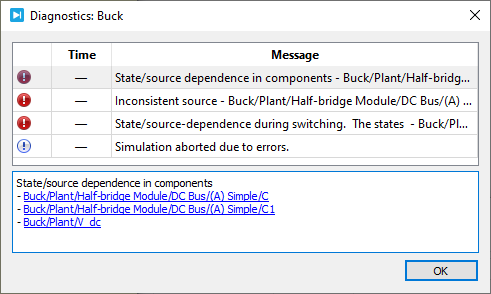
There are two ways of solving this issue:

1. Use the (B) Detailed level instead for the power modules directly in parallel with a voltage source.
2. Insert a small resistor (typically a few milliohms) in series with the DC source. However, the resistance must be chosen carefully so that it does not significantly affect the system dynamics (if it is too large) or cause numerical problems (if it is too small).

Compatibility with HIL simulation

The PLECS blocks in the Imperix Power library are compatible with the Hardware-in-the-loop (HIL) simulation using the Plexim RT-Box (using Plexim’s sub-cycle average model). The PLECS_RT_Box target support package is also required for HIL use.

Specialized Power System library removed in MATLAB R2026a

Starting with MATLAB R2026a, the Specialized Power Systems library (the “Black” blocks) has been removed from Simscape Electrical. Its functionality has been moved to OPAL-RT’s SPS Software, which requires a separate paid license.

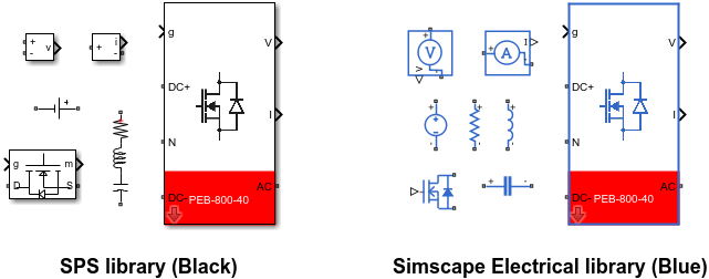
In response to this change, imperix has separated the Power library for Simulink into two distinct libraries: Imperix Power (SPS) and Imperix Power (Simscape Electrical). This update is included in ACG SDK 2026.1.3 and newer versions (available to download here). More information about this situation is given in our blog article.

• Users who want to keep using the SPS library (the “black” blocks) in MATLAB R2026a and newer versions will need to contact OPAL-RT for an SPS Software license.
• Users who want to switch to Simscape Electrical (the “blue” blocks) will need to switch to the Imperix Power (Simscape Electrical) library.

Getting started example: three-phase PV inverter simulation

The Simulink and PLECS models provided below implement a three-phase PV inverter, where the plant model is built with blocks from the Imperix Power library. The controller model is the same as the one in AN006.

The file below contains the PLECS model with a Hardware-In-the-Loop (HIL) configuration that can be used with the B-Box 3 together with an RT-Box.

The file below contains the plant model built with Simscape Electrical. The control model remains the same.

The example models have the following simulation scenario, which is illustrated by the results below:

• At t=0, the DC bus is already precharged at 500V and the PWMs are not yet activated.
• At t=0.1s, the “activate” variable is set to 1. The PWMs are immediately activated (FSM is bypassed in simulation), the DC bus voltage is regulated at 750V, and the MPPT algorithm converges gradually to the MPP (corresponding to a PV current reference around 18A).
  After the MPPT algorithm has converged (after t=0.22s), the Perturb and Observe algorithm gives a PV current reference that oscillates around the MPP current.
• At t=0.5s, the DC voltage reference is reduced to 700V.
• At t=0.8s, the solar irradiance is reduced (simulation of passing clouds). The MPPT algorithm gradually decreases the PV current reference and reaches the new MPP at around t=1s (corresponding to a PV current reference around 15A).

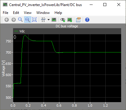
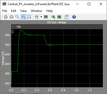
The simulation time in PLECS is shown below. For a control running at 20kHz, there is almost no visible difference between the waveforms under different configurations. On the other hand, the simulation time can be significantly reduced by choosing an appropriate plant model. Overall, for most applications, it is recommended to use (A) Simple modeling level and averaged model together with duty-cycle outputs of CB-PWM to achieve fast and accurate simulation.

A similar and more complete benchmark is given in TN182, also addressing how to improve simulation speed using Simscape Electrical.

Model configuration	Simulation time [s]
(A) Simple, switched	38.7
(B) Detailed, switched	62.2
(A) Simple, averaged	8.42
(B) Detailed, averaged	8.67

To go further

More examples are available on the knowledge base, covering a wide range of application scenarios.

• AN015 – Solid-state transformer (SST) for MV-LV smart grids
• TN132 – Getting started with an NPC converter
• TN138 – V/f control of an induction machine
• TN167 – Grid-Following Inverter (GFLI)